Pre-lecture materials
Acknowledgements
Material for this lecture was borrowed and adopted from
- An Introduction to Statistical Learning, 2nd edition by James, Witten, Hastie and Tibshirani
- https://jhu-advdatasci.github.io/2019/
Learning objectives
At the end of this lesson you will:
- Understand what are hyperplanes, maximal margin hyperplanes, support vector classifiers (with and without linear boundaries), and Support Vector Machines (SVM)
- Know how to build a SVM with the
caretR package
Motivation
In this lecture, we will be asking the question:
Can we identify a voice as male or female, based upon acoustic properties of the voice and speech?
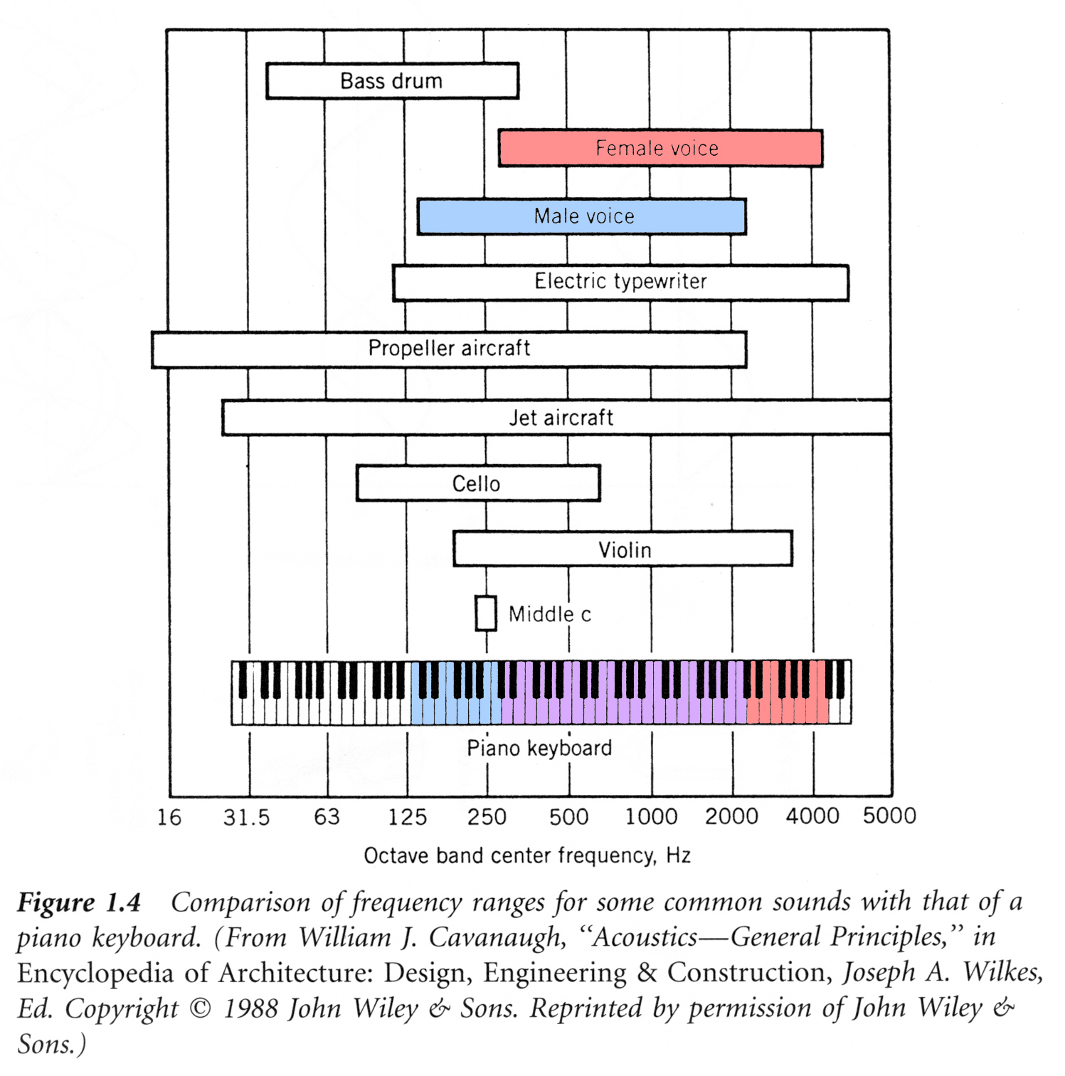
Determining a person’s gender as male or female, based upon a sample of their voice seems to initially be a feasible task. Often, the human ear can detect the difference between a male or female voice within the first few spoken words. However, designing a computer program to do this turns out to be a bit trickier.
To accomplish that goal, we will learn about another machine learning algorithm called support vector machines (SVMs). SVMs have been around since the 1990s and originated of the computer science community. They are form of supervised learning.
SVMs are widely applied to pattern classification and regression problems, such as:
- Handwritten digits classification
- Speech recognition
- Facial expression classification
- Text classification
The original idea was to build a classifier for which training data can be separated using some type of linear hyperplane. We want a hyperplane that maximizes the distance between the hyperplane to the nearest data point in either class.
In the case when we cannot draw a linear hyperplane to separate the two classes of points (this is more typical), we can adapt the idea and build a non-linear classifier. The key idea is to apply a “kernel trick”. We’ll learn more about that later in the lecture.
Note: We will focus on the case when there are only two classes, but there are also extensions of SVMs in the case when there are more than two classes.
How does it work?
Given a dataset with a set of features and set of labels, we want to build a support vector machine (SVMs) to predict classes for new observations.
To understand what is a SVM let’s build up to it and consider some other types of classifiers (or hyperplanes) and how it relates to SVMs. First, let’s use a plain ole hyperplane.
Hyperplanes
A hyperplane is formally defined as a flat affine subspace of a dimension \(p-1\).
For example, in two dimensions, a hyperplane is a flat one-dimensional subspace (or a line). In this case, a hyperplane is defined by
\[ \beta_0 + \beta_1 X_1 + \beta_2 X_2 = 0 \]
for \(X = (X_1, X_2)^{T}\) and for parameters \(\beta_0\), \(\beta_1\) and \(\beta_2\). If there are \(X = (X_1, X_2)^{T}\) that do not satisify the above, i.e
\[ \beta_0 + \beta_1 X_1 + \beta_2 X_2 > 0 \]
or
\[ \beta_0 + \beta_1 X_1 + \beta_2 X_2 < 0 \]
Then, we can think of the hyperplane as dividing the two-dimensional space into two halves.
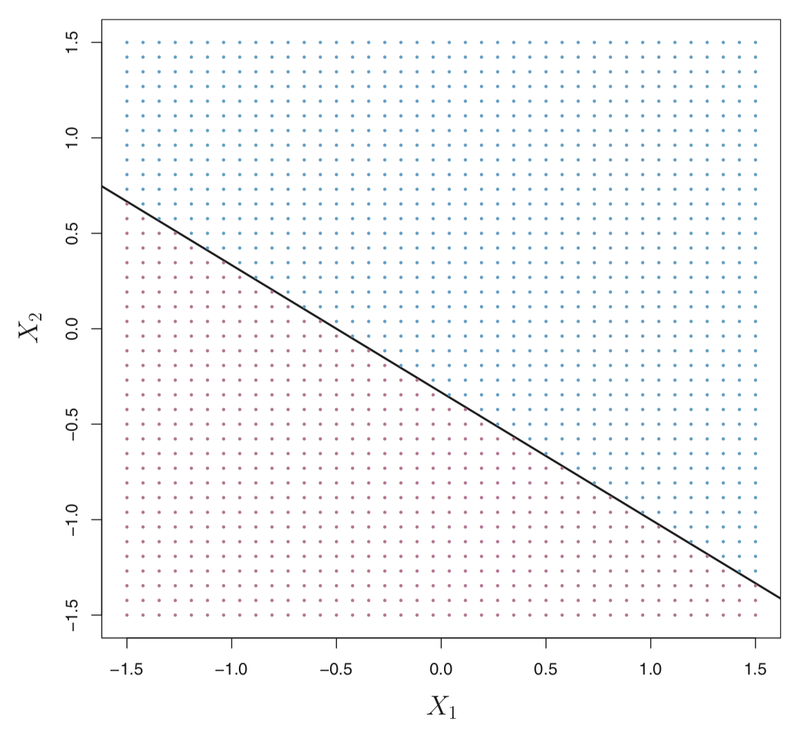
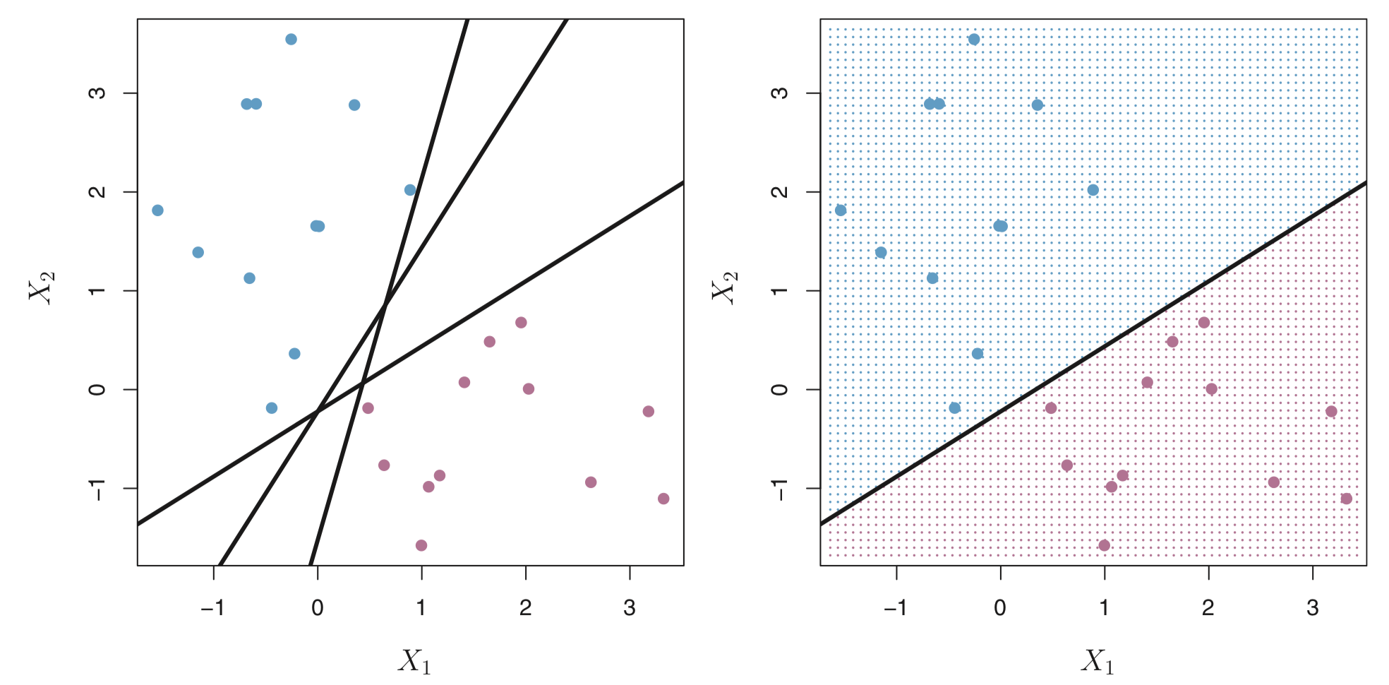
In the figure below, the hyperplane \(1 + 2X_1 + 3X_2 = 0\) is shown. The set of points in the blue region is \(1 + 2X_1 + 3X_2 > 0\) and the purple region is the set of points for which \(1 + 2X_1 + 3X_2 < 0\).
More formally, let’s say we have a set of \(n\) training observations \(X_i = (X_{i1}, X_{i2})^T\) in with two features (\(p=2\)) and each training observation has a known label \(y_i \in \{-1,1\}\) where the observations from the blue class are labeled as \(y_i = 1\) and those from the purple class are \(y_i = -1\).
A hyperplane that separates the observations
\[ \beta_0 + \beta_1 X_1 + \beta_2 X_2 > 0 \text{ if } y_i = 1 \]
or
\[ \beta_0 + \beta_1 X_1 + \beta_2 X_2 < 0 \text{ if } y_i = -1 \] or
\[ y_i (\beta_0 + \beta_1 X_1 + \beta_2 X_2) < 0 \text{ for all } i\in(1, \ldots, n) \]
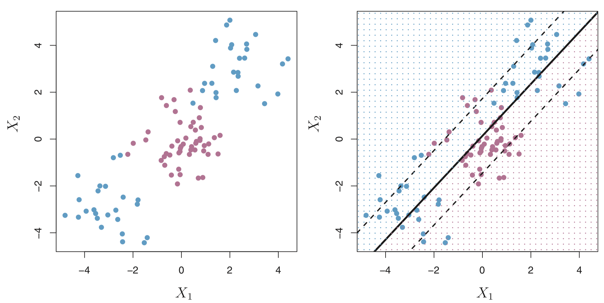
There can be many hyperplanes that separate these points in our example. For example, the figure on the left shows three hyperplanes in black (out of many). If we pick one hyperplane, the figure on the right shows a grid of blue an purple points indicating the decision rule made by a classifer defined by this hyperplane.
More formally, we can classify a test observation \(x^{*}\) based on the sign of of
\[ f(x^{*}) = \beta_0 + \beta_1 x_1^{*} + \beta_2 x_2^{*} \]
- If \(f(x^{*})\) is positive, then we assign \(x^{*}\) to the blue class.
- If \(f(x^{*})\) is negative, then we assign \(x^{*}\) to the purple class.
In addition to the sign, we can also consider the magnitude of \(f(x^{*})\).
- If \(f(x^{*})\) is far from zero, then \(x^{*}\) is far away from the hyperplane (i.e. more confidence in our class assignment).
- If \(f(x^{*})\) is close to zero, then \(x^{*}\) is close to the hyperplane (i.e. less certain about the class assignment for \(x^{*}\)).
But, the problem is this still can lead to an infinite number of possible separating hyperplanes. How can we decide what is the “best” hyperplane?
Maximal Margin Hyperplane (or Classifer)
The maximal margin hyperplane is the hyperlane that separates the farthest from training observations.
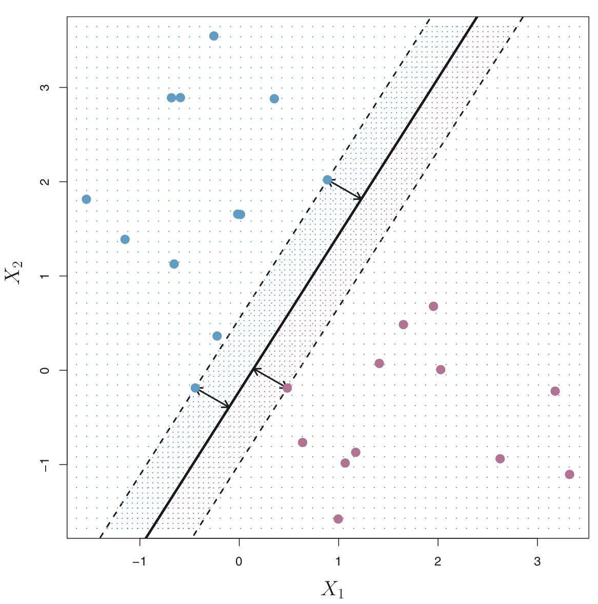
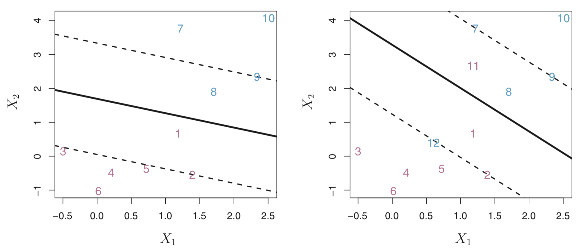
In the figure below, the maximal margin hyperplane is shown as a solid line.
The margin is the distance from the solid line to either of the dashed lines.
The two blue points and the purple point that lie on the dashed lines are the support vectors (they “support” the maximal margin hyperplane in the sense that if these points were moved slightly then the maximal margin hyperplane would move as well), and the distance from those points to the margin is indicated by arrows.
The purple and blue grid indicates the decision rule made by a classifier based on this separating hyperplane.
This is a really power idea and this is what SVMs are built on. BUT
Pro tip: Although the maximal margin classifier is often successful, it can also lead to overfitting when \(p\) is large. So if you use this, it’s important to explore the use of cross-validation.
To construct a maximal margin classifier using \(n\) training observations \(x_1, \ldots, x_n \in \mathbb{R}^p\) and associated class labels \(y_1 \ldots, y_n \in \{-1, 1\}\), the maximal margin hyperplane is the solution to the optimization problem:
\[ \underset{\beta_0, \beta_1, \ldots, \beta_p, M}{\text{maximize }} M \] subject to \(\sum_{j=1}^p \beta_j^2 = 1\) and
\[ y_i (\beta_0 + \beta_1 x_1 + \ldots + \beta_p x_p) \geq M \text{ for all } i\in(1, \ldots, n) \]
Note:
SVM uses L2 regularization on the \(\beta\) coefficients (like ridge regression) vs L1 regularization (like in Lasso regression)
L1 regularization might be better / less susceptible to outliers. In fact there are L1 SVMs
This guarantees that each observation will be on the correct side of the hyperplane and at least a distance of \(M\) from the hyperplane. Therefore, you can think of \(M\) as the margin of our hyperplane.
This works great if a separating hyperplane exists. However, many times, that isn’t true and there is no solution with \(M > 0\). So instead we can try to find a hyperplane that almost separates the classes (with some penalty or cost associated with each observation that is is on the wrong side of the hyperplane).
Support Vector Classifer
Consider the following data that cannot be separated by a hyperplane.
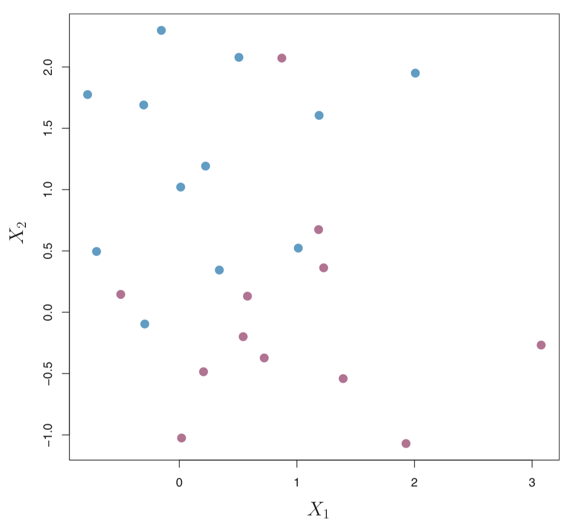
We could consider building a support vector classifer or a soft margin classifer that misclassifies a few training observations in order to do a better job of classifying the remaining observations.
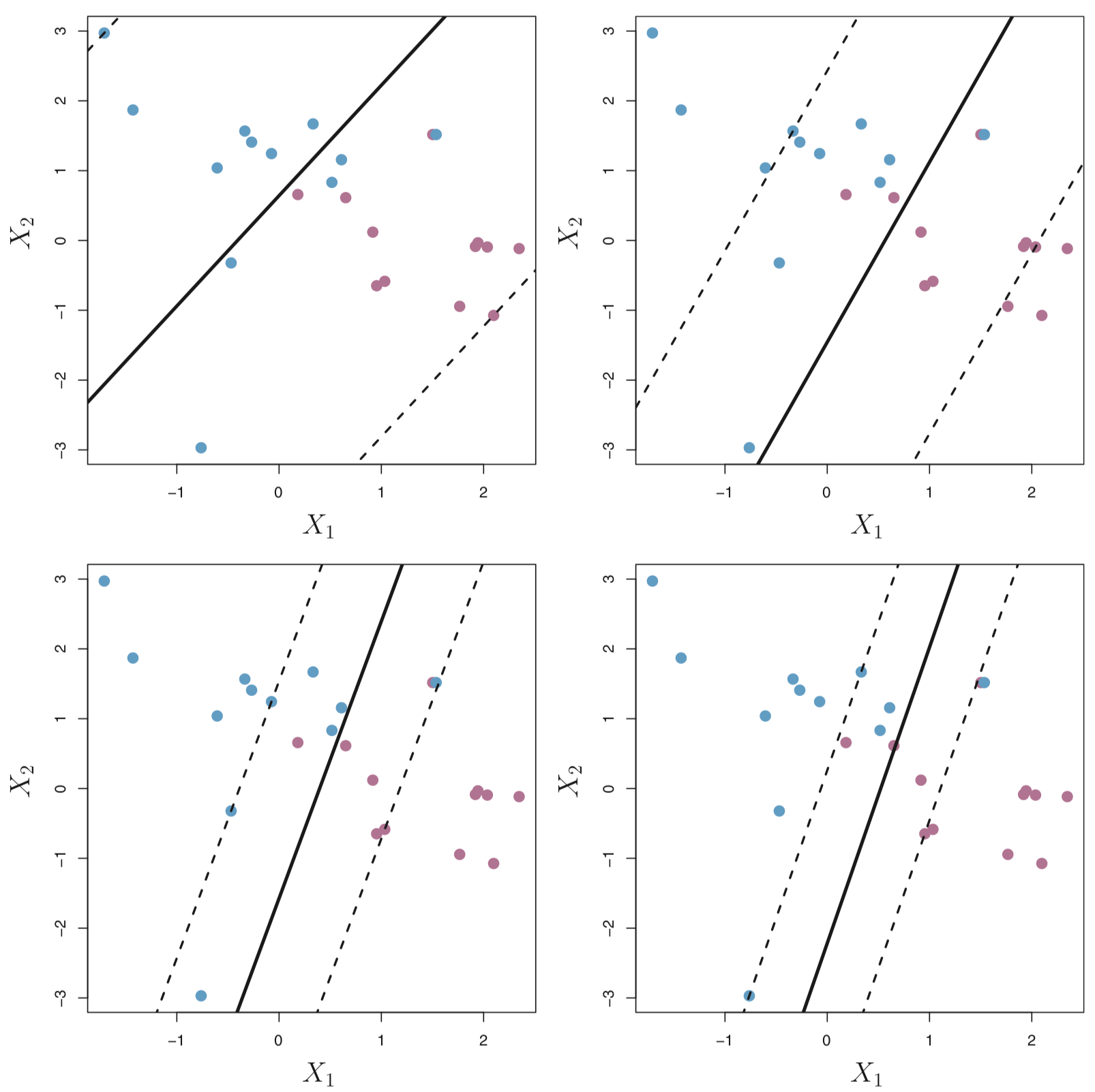
The margin is soft because it can be violated by some of the training observations. An observation can be not only on the wrong side of the margin, but also on the wrong side of the hyperplane.
On the left there are observations that are on the right side of the hyperplane, but the wrong side of the margin. On the right are observations that are on the wrong side of the hyperplane and the wrong side of the margin.
In fact, when there is no separating hyperplane, such a situation is inevitable. Observations on the wrong side of the hyperplane correspond to training observations that are misclassified by the support vector classifier (i.e. right figure above).
Now, the optimization problem is:
\[ \underset{\beta_0, \beta_1, \ldots, \beta_p, \epsilon_1, \ldots, \epsilon_n, M}{\text{maximize}} M \] subject to \(\sum_{j=1}^p \beta_j^2 = 1\)
\[ y_i (\beta_0 + \beta_1 x_1 + \ldots + \beta_p x_p) \geq M (1-\epsilon_i) \] for all \(i\in(1, \ldots, n)\), \(\epsilon_i \geq 0\), \(\sum_{i=1}^n \epsilon_i \leq C\) where \(C\) is a nonnegative tuning parameter (typically chosen using cross-validation). The \(\epsilon_1, \ldots, \epsilon_n\) are often called slack variables that allow observations to be on the wrong side of the margin or hyperplane.
Note:
- L2 regularization in SVMs is imposes a bigger (quadratic vs linear) loss for points that violate the margin in SVMs
Comments on the tuning parameter \(C\)
We see that \(C\) bounds the sum of the \(\epsilon_i\)’s, so you think about it as a “budget” for the amount of margin that can be violated in the \(n\) observations.
- If \(C = 0\) \(\Rightarrow\) No budget for violations to the margin and \(\epsilon_1 = \ldots = \epsilon_n = 0\). This is essentially the maximal margin hyperplane (but only if the two classes are separable).
- If \(C > 0\) \(\Rightarrow\) No more than \(C\) observations can be on the wrong side of the hyperplane, because if an observation is on the wrong side of the hyperplane then \(\epsilon_i > 1\), and we saw above, this requires that \(\sum_{i=1}^n \epsilon_i \leq C\).
In general, as the budget \(C\) increases, we become more tolerant of violations to the margin, and so the margin will widen. Conversely, as \(C\) decreases, we become less tolerant of violations to the margin and so the margin narrows.
Another way of thinking about \(C\) is that it basically controls the bias-variance trade-off.
- When \(C\) is small, we seek narrow margins that are rarely violated; this amounts to a classifier that is highly fit to the data, which may have low bias but high variance.
- When \(C\) is larger, the margin is wider and we allow more violations to it; this amounts to fitting the data less hard and obtaining a classifier that is potentially more biased but may have lower variance.
Interestingly, it turns out that only the observations that lie on the margin or that violate the margin (also known as support vectors) will affect the hyperplane (and hence classification).
This make sense. But why?
When \(C\) is large, the margin is wide, and many observations violate the margin, thus there are many support vectors (potentially more bias, but less variance). When \(C\) is small, the margin is small, not many observations violate the margin, thus very few support vectors (potentially low bias and high variance).
OK, but what if we want to consider non-linear boundaries?
Support Vector Classifier with Non-Linear boundaries
Thus far, the support vector classifier has been very useful for classification in the setting with two classes and if the classes can be separated by a linear hyperplane (with or without some violations of margins of error). However, more often than not, the boundry will need to be more flexible and consider non-linear class boundaries.
Consider the following data on the left plot. A linear support classifier (applied in the right plot) will perform poorly.
When using linear regression, if there is a non-linear relationship between the predictors and outcome, a solution is to enlarge the feature space to include e.g. quadratic and cubic terms
Therefore, a solution to our problem is to enlarge the feature space using functions of the predictors (i.e. quadratic and cubic terms or higher) in order to address the non-linearity.
So instead of fitting a support vector classifier with \(p\) features \((X_1, X_2, \ldots, X_p)\), we could try using \(2p\) features \((X_1, X_1^2, X_2, X_2^2, \ldots, X_p, X_p^2)\).
Now, the optimization problem becomes:
\[ \underset{\beta_0, \beta_{11}, \beta_{12}, \ldots, \beta_{p1}, \beta_{p2}, \epsilon_1, \ldots, \epsilon_n, M}{\text{maximize}} M \] subject to
\[ y_i (\beta_0 + \sum_{j=1}^p \beta_{j1} x_{ij} + \sum_{j=1}^p \beta_{j2} x_{ij}^2) \geq M (1-\epsilon_i) \] \(\sum_{i=1}^n \epsilon_i \leq C\), \(\epsilon_i \geq 0\), \(\sum_{j=1}^p \sum_{k=1}^2 \beta_{jk}^2 = 1\)
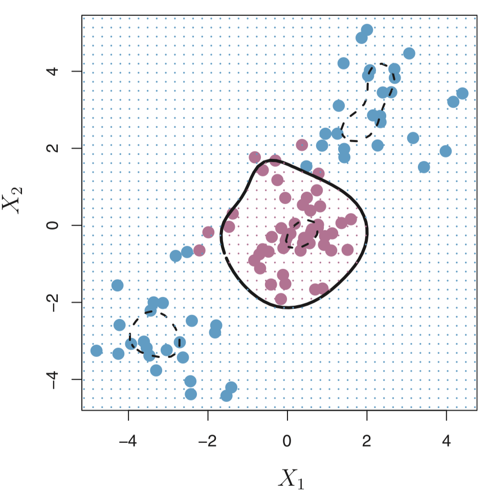
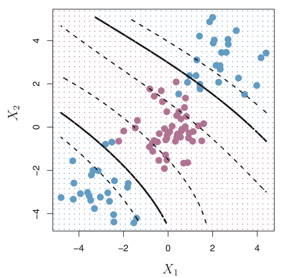
Why does this lead to a non-linear boundary?
In the enlarged feature space, the decision boundary that is found is still linear. But in the original feature space, the decision boundary is of the form \(q(x) = 0\), where \(q\) is a quadratic polynomial, and its solutions are generally non-linear.
As you can imagine, there are many ways to enlarge the feature space e.g. include higher-order polynomial terms or interaction terms such as \(X_1 X_2\). We could easily end up with a large number of features leading to unmanagable computations.
In the next section, we will learn about the support vector machine that allows us to enlarge the feature space in an efficient way.
Support Vector Machines
The support vector machine (SVM) is an extension of the support vector classifier that results from enlarging the feature space in a specific way, using kernels.
The details of how exactly how the support vector classifier is computed is quite technical, so I won’t go into it here. However, it’s sufficient to know that the solution to the support vector classifier problem involves only the inner products of the observations (as opposed to the observations themselves). The inner product of two observations \(x_i\) and \(x_{i^{'}}\) is given by
\[ \langle x_i, x_{i^{'}} \rangle = \sum_{j=1}^P x_{ij} x_{i^{'}j}\]
For example, the linear support vector classifier can be represented as
\[ f(x) = \beta_0 + \sum_{i=1}^n \alpha_i \langle x, x_{i} \rangle \]
where there are \(n\) parameters \(\alpha_i\) (one per training observation).
To estimate the parameters \(\alpha_1, \ldots, \alpha_n\) and \(\beta_0\), we need to take \({n \choose 2}\) inner products between all pairs of training observations \(x_i\) and \(x_{i^{'}}\).
To evaluate the function \(f(x)\), all we need is the inner product between a new point \(x\) and each of the training points \(x_i\). Interestingly, it turns out that \(\alpha_i\) is nonzero only for the support vectors (points in the margin). Another way of stating this is if a training observation is not a support vector, then its \(\alpha_i\) is equals zero.
So if we consider \(\mathcal{S}\) as the collection of indicies for support points, then we can rewrite the above to
\[ f(x) = \beta_0 + \sum_{i \in \mathcal{S}} \alpha_i \langle x, x_{i} \rangle \] And this involves a lot fewer points!
Ok, now suppose that instead of the inner product, we consider a generalization of the inner product of the form
\[ K( x_i, x_{i^{'}} ) \]
where \(K\) is some function called a kernel.
You can think of a kernel as a function that quantifies the similiarity of two observations. For example,
\[ K( x_i, x_{i^{'}} ) = \sum_{j=1}^p x_{ij} x_{i^{'}j} \]
is a linear kernel (linear in the features) and would return the support vector classifier.
In contrast, this kernel is called a polynomial kernel of degree \(d\). If \(d > 1\), then the support vector classifier results in a more flexible boundary.
\[ K( x_i, x_{i^{'}} ) = \Big(1 + \sum_{j=1}^p x_{ij} x_{i^{'}j} \Big)^d \]
When the support vector classifier is combined with non-linear kernels (such as above), the resulting classifier is known as a support vector machine.
Another popular kernel is the radial kernel:
\[ K( x_i, x_{i^{'}} ) = \exp \Big(-\gamma \sum_{j=1}^p (x_{ij} - x_{i^{'}j})^2 \Big) \]
Advantages
- SVMs are effective when the number of features is quite large.
- It works effectively even if the number of features are greater than the number of samples.
- Non-Linear data can also be classified using customized hyperplanes built by using kernel trick.
- It is a robust model to solve prediction problems since it maximizes margin.
Disadvantages
- The biggest limitation of SVMs is the choice of the kernel. The wrong choice of the kernel can lead to an increase in error percentage.
- With a greater number of samples, it can result in poor performance.
- SVMs have good generalization performance but they can be extremely slow in the test phase.
- SVMs have high algorithmic complexity and extensive memory requirements due to the use of quadratic programming.
Let’s try out these concepts on the data from our original question:
Can we identify a voice as male or female, based upon acoustic properties of the voice and speech?
Data
The data we will use is from kaggle and is available in a .csv file.
A description of the data from Kaggle:
“This database was created to identify a voice as male or female, based upon acoustic properties of the voice and speech. The dataset consists of 3,168 recorded voice samples, collected from male and female speakers. The voice samples are pre-processed by acoustic analysis in R using the seewave and tuneR packages.”
We can actually dig a bit deeper and go to the website where the data origianlly came from to learn more about how the dataset was created:
“Each voice sample is stored as a
.WAVfile, which is then pre-processed for acoustic analysis using the specan function from the WarbleR R package. Specan measures 22 acoustic parameters on acoustic signals for which the start and end times are provided.”
“The output from the pre-processed WAV files were saved into a CSV file, containing 3168 rows and 21 columns (20 columns for each feature and one label column for the classification of male or female).”
The following acoustic properties of each voice are measured (described on Kaggle’s website):
| Variable | Description |
|---|---|
meanfreq |
mean frequency (in kHz) |
sd |
standard deviation of frequency |
median |
median frequency (in kHz) |
Q25 |
first quantile (in kHz) |
Q75 |
third quantile (in kHz) |
IQR |
interquantile range (in kHz) |
skew |
skewness |
kurt |
kurtosis |
sp.ent |
spectral entropy |
sfm |
spectral flatness |
mode |
mode frequency |
centroid |
frequency centroid |
peakf |
peak frequency (frequency with highest energy) |
meanfun |
average of fundamental frequency measured across acoustic signal |
minfun |
minimum fundamental frequency measured across acoustic signal |
maxfun |
maximum fundamental frequency measured across acoustic signal |
meandom |
average of dominant frequency measured across acoustic signal |
mindom |
minimum of dominant frequency measured across acoustic signal |
maxdom |
maximum of dominant frequency measured across acoustic signal |
dfrange |
range of dominant frequency measured across acoustic signal |
modindx |
modulation index. Calculated as the accumulated absolute difference between adjacent measurements of fundamental frequencies divided by the frequency range |
label |
male or female |
Import data
First, we load a few R packages
Let’s read in the voice.csv file into R using the read_csv() function in the readr R package.
voice <- read_csv(here("data", "voice.csv"))
voice
# A tibble: 3,168 × 21
   meanfreq     sd median     Q25    Q75    IQR  skew    kurt sp.ent
      <dbl>  <dbl>  <dbl>   <dbl>  <dbl>  <dbl> <dbl>   <dbl>  <dbl>
 1   0.0598 0.0642 0.0320 0.0151  0.0902 0.0751 12.9   274.    0.893
 2   0.0660 0.0673 0.0402 0.0194  0.0927 0.0733 22.4   635.    0.892
 3   0.0773 0.0838 0.0367 0.00870 0.132  0.123  30.8  1025.    0.846
 4   0.151  0.0721 0.158  0.0966  0.208  0.111   1.23    4.18  0.963
 5   0.135  0.0791 0.125  0.0787  0.206  0.127   1.10    4.33  0.972
 6   0.133  0.0796 0.119  0.0680  0.210  0.142   1.93    8.31  0.963
 7   0.151  0.0745 0.160  0.0929  0.206  0.113   1.53    5.99  0.968
 8   0.161  0.0768 0.144  0.111   0.232  0.121   1.40    4.77  0.959
 9   0.142  0.0780 0.139  0.0882  0.209  0.120   1.10    4.07  0.971
10   0.134  0.0804 0.121  0.0756  0.202  0.126   1.19    4.79  0.975
# … with 3,158 more rows, and 12 more variables: sfm <dbl>,
#   mode <dbl>, centroid <dbl>, meanfun <dbl>, minfun <dbl>,
#   maxfun <dbl>, meandom <dbl>, mindom <dbl>, maxdom <dbl>,
#   dfrange <dbl>, modindx <dbl>, label <chr>
Next, let’s get an overall summary of the range of values in the dataset.
summary(voice)
    meanfreq             sd              median
 Min.   :0.03936   Min.   :0.01836   Min.   :0.01097
 1st Qu.:0.16366   1st Qu.:0.04195   1st Qu.:0.16959
 Median :0.18484   Median :0.05916   Median :0.19003
 Mean   :0.18091   Mean   :0.05713   Mean   :0.18562
 3rd Qu.:0.19915   3rd Qu.:0.06702   3rd Qu.:0.21062
 Max.   :0.25112   Max.   :0.11527   Max.   :0.26122
      Q25                 Q75               IQR
 Min.   :0.0002288   Min.   :0.04295   Min.   :0.01456
 1st Qu.:0.1110865   1st Qu.:0.20875   1st Qu.:0.04256
 Median :0.1402864   Median :0.22568   Median :0.09428
 Mean   :0.1404556   Mean   :0.22476   Mean   :0.08431
 3rd Qu.:0.1759388   3rd Qu.:0.24366   3rd Qu.:0.11418
 Max.   :0.2473469   Max.   :0.27347   Max.   :0.25223
      skew              kurt              sp.ent
 Min.   : 0.1417   Min.   :   2.068   Min.   :0.7387
 1st Qu.: 1.6496   1st Qu.:   5.670   1st Qu.:0.8618
 Median : 2.1971   Median :   8.319   Median :0.9018
 Mean   : 3.1402   Mean   :  36.569   Mean   :0.8951
 3rd Qu.: 2.9317   3rd Qu.:  13.649   3rd Qu.:0.9287
 Max.   :34.7255   Max.   :1309.613   Max.   :0.9820
      sfm               mode           centroid
 Min.   :0.03688   Min.   :0.0000   Min.   :0.03936
 1st Qu.:0.25804   1st Qu.:0.1180   1st Qu.:0.16366
 Median :0.39634   Median :0.1866   Median :0.18484
 Mean   :0.40822   Mean   :0.1653   Mean   :0.18091
 3rd Qu.:0.53368   3rd Qu.:0.2211   3rd Qu.:0.19915
 Max.   :0.84294   Max.   :0.2800   Max.   :0.25112
    meanfun            minfun             maxfun
 Min.   :0.05557   Min.   :0.009775   Min.   :0.1031
 1st Qu.:0.11700   1st Qu.:0.018223   1st Qu.:0.2540
 Median :0.14052   Median :0.046110   Median :0.2712
 Mean   :0.14281   Mean   :0.036802   Mean   :0.2588
 3rd Qu.:0.16958   3rd Qu.:0.047904   3rd Qu.:0.2775
 Max.   :0.23764   Max.   :0.204082   Max.   :0.2791
    meandom             mindom             maxdom
 Min.   :0.007812   Min.   :0.004883   Min.   : 0.007812
 1st Qu.:0.419828   1st Qu.:0.007812   1st Qu.: 2.070312
 Median :0.765795   Median :0.023438   Median : 4.992188
 Mean   :0.829211   Mean   :0.052647   Mean   : 5.047277
 3rd Qu.:1.177166   3rd Qu.:0.070312   3rd Qu.: 7.007812
 Max.   :2.957682   Max.   :0.458984   Max.   :21.867188
    dfrange          modindx           label
 Min.   : 0.000   Min.   :0.00000   Length:3168
 1st Qu.: 2.045   1st Qu.:0.09977   Class :character
 Median : 4.945   Median :0.13936   Mode  :character
 Mean   : 4.995   Mean   :0.17375
 3rd Qu.: 6.992   3rd Qu.:0.20918
 Max.   :21.844   Max.   :0.93237
A quick glimpse over the data shows us that we have 20 numeric columns with differing ranges and magnitudes.
Wrangling data
It would be nice to get a picture of how these features are different across the male and female observations. One way to do that is to use ggplot() to explore differences in distribution with boxplots and histograms.
First, let’s transform the data from a wide format to a long format using the pivot_longer() function in the tidyr package.
voice_long <- voice %>%
  pivot_longer(cols = -label, names_to = "feature", values_to = "value")

head(voice_long)
# A tibble: 6 × 3
  label feature   value
  <chr> <chr>     <dbl>
1 male  meanfreq 0.0598
2 male  sd       0.0642
3 male  median   0.0320
4 male  Q25      0.0151
5 male  Q75      0.0902
6 male  IQR      0.0751
We also can transform the label column which contains male and female character strings into 1s and 0s where 1 represents male and 0 represents `female.
table(voice$label)
female   male
1584 1584 Just as a sanity check:
table(voice_labels, voice$y)
voice_labels    0    1
      female 1584    0
      male      0 1584
Whew ok good!
EDA
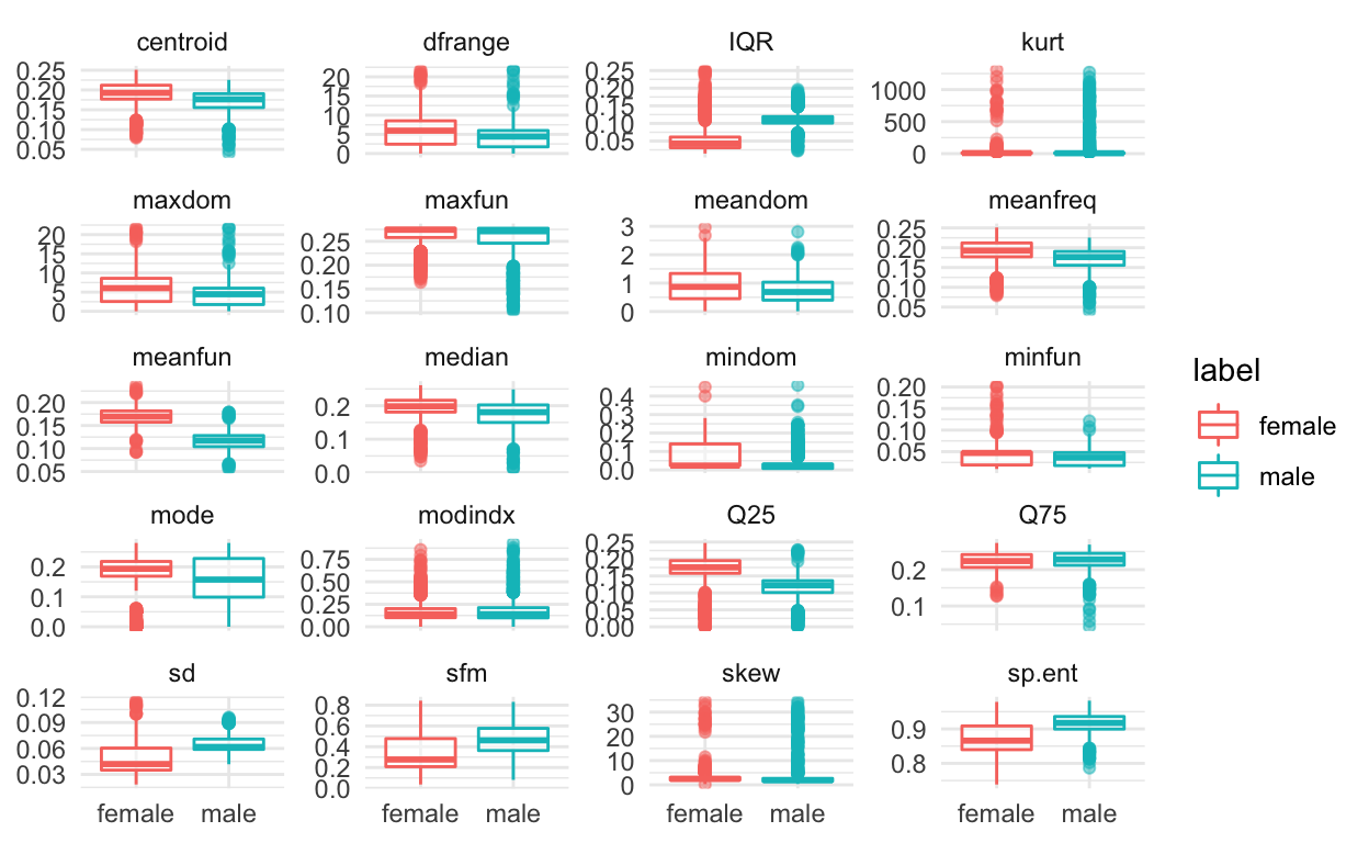
If we wanted to create boxplots of all twenty variables colored by whether the observation was male or female, we can use the
voice_long %>%
    ggplot(aes(label, value, colour = label)) +
        geom_boxplot(alpha = 0.5) +
        facet_wrap(~ feature, scales='free_y', ncol = 4) +
        labs(x = NULL, y = NULL) +
        theme_minimal()
voice_long %>%
    ggplot(aes(value, fill = label)) +
        geom_density(alpha = 0.5) +
        facet_wrap(~ feature, scales='free', ncol = 4) +
        labs(x = NULL, y = NULL) +
        theme_minimal()
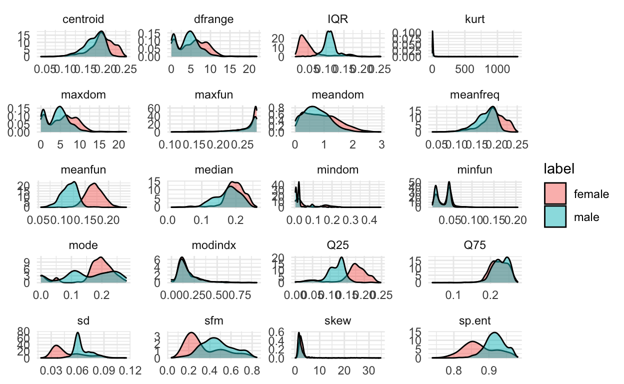
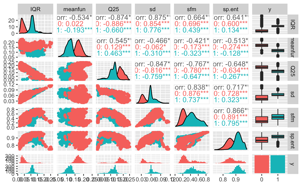
These are great to look at the distributions separately, but it would also be good to get an idea of how the features are related to each other.
To do that, another useful plotting function for exploratory data analysi is the ggpairs() function from the GGally package:
Classification models
Next, we will build a few models to classify the recorded voice samples as male or female using features available. First, we will look at SVMs and then we will compare to other models that we have already seen that are useful for classification including logistic regression and random forests.
Support Vector Machines
Before we build an SVM classifier, let’s split our data into a train_set and test_set using the createDataParition() function in the caret R package.
We’ll just split it in half for the purposes of the lecture.
set.seed(1234)
set.seed(1234)
train_set = createDataPartition(y = voice$y,
                                p = 0.5, list=FALSE)

train_dat = voice[train_set,]
test_dat = voice[-train_set,]
We can look at the dimensions of the two datasets to make sure they have been split in half.
And they have! Ok, before we build a SVM using train() function (we’ve seen this before), let’s use the trainControl() function. Here, we select method=cv with 10-fold cross-validation.
control <- trainControl(method="cv", number=10)
metric <- "Accuracy"
SVM with linear kernel
First, we will use the train() function from the caret R package with the argument method=svmLinear to build a SVM with linear kernel.
fit_svmLinear <- train(y~., data=train_dat, method="svmLinear",
                metric=metric, trControl=control)
fit_svmLinear
Support Vector Machines with Linear Kernel

1584 samples
  20 predictor
   2 classes: '0', '1'

No pre-processing
Resampling: Cross-Validated (10 fold)
Summary of sample sizes: 1424, 1426, 1426, 1425, 1426, 1426, ...
Resampling results:

  Accuracy   Kappa
  0.9722233  0.9444468

Tuning parameter 'C' was held constant at a value of 1
newdata <- as.data.frame(select(train_dat, -y))
pred_svmLinear <- predict(fit_svmLinear, newdata)
confusionMatrix(reference=train_dat$y, pred_svmLinear)
Confusion Matrix and Statistics

          Reference
Prediction   0   1
         0 775  19
         1  17 773

               Accuracy : 0.9773
                 95% CI : (0.9687, 0.984)
    No Information Rate : 0.5
    P-Value [Acc > NIR] : <2e-16

                  Kappa : 0.9545

 Mcnemar's Test P-Value : 0.8676

            Sensitivity : 0.9785
            Specificity : 0.9760
         Pos Pred Value : 0.9761
         Neg Pred Value : 0.9785
             Prevalence : 0.5000
         Detection Rate : 0.4893
   Detection Prevalence : 0.5013
      Balanced Accuracy : 0.9773

       'Positive' Class : 0
SVM with polynomial kernel
Next, we will use the train() function from the caret R package with the argument method=svmPoly to build a SVM with polynomial kernel.
fit_svmPoly <- train(y~., data=train_dat, method="svmPoly",
                metric=metric, trControl=control)
fit_svmPoly
Support Vector Machines with Polynomial Kernel

1584 samples
  20 predictor
   2 classes: '0', '1'

No pre-processing
Resampling: Cross-Validated (10 fold)
Summary of sample sizes: 1425, 1425, 1426, 1426, 1426, 1425, ...
Resampling results across tuning parameters:

  degree  scale  C     Accuracy   Kappa
  1       0.001  0.25  0.8876682  0.7752831
  1       0.001  0.50  0.8965130  0.7929541
  1       0.001  1.00  0.9123079  0.8245470
  1       0.010  0.25  0.9318884  0.8637212
  1       0.010  0.50  0.9564923  0.9129594
  1       0.010  1.00  0.9653372  0.9306550
  1       0.100  0.25  0.9684818  0.9369517
  1       0.100  0.50  0.9684738  0.9369354
  1       0.100  1.00  0.9728923  0.9457742
  2       0.001  0.25  0.8965130  0.7929541
  2       0.001  0.50  0.9116750  0.8232812
  2       0.001  1.00  0.9262081  0.8523590
  2       0.010  0.25  0.9634344  0.9268506
  2       0.010  0.50  0.9672160  0.9344180
  2       0.010  1.00  0.9691028  0.9381925
  2       0.100  0.25  0.9690829  0.9381582
  2       0.100  0.50  0.9716105  0.9432131
  2       0.100  1.00  0.9722474  0.9444863
  3       0.001  0.25  0.9078776  0.8156823
  3       0.001  0.50  0.9205278  0.8409935
  3       0.001  1.00  0.9413622  0.8826757
  3       0.010  0.25  0.9672160  0.9344182
  3       0.010  0.50  0.9691028  0.9381941
  3       0.010  1.00  0.9678370  0.9356624
  3       0.100  0.25  0.9690789  0.9381492
  3       0.100  0.50  0.9716066  0.9432057
  3       0.100  1.00  0.9747632  0.9495179

Accuracy was used to select the optimal model using the
 largest value.
The final values used for the model were degree = 3, scale = 0.1
 and C = 1.
newdata <- as.data.frame(select(train_dat, -y))
pred_svmPoly <- predict(fit_svmPoly, newdata)
confusionMatrix(reference=train_dat$y, pred_svmPoly)
Confusion Matrix and Statistics

          Reference
Prediction   0   1
         0 789   3
         1   3 789

               Accuracy : 0.9962
                 95% CI : (0.9918, 0.9986)
    No Information Rate : 0.5
    P-Value [Acc > NIR] : <2e-16

                  Kappa : 0.9924

 Mcnemar's Test P-Value : 1

            Sensitivity : 0.9962
            Specificity : 0.9962
         Pos Pred Value : 0.9962
         Neg Pred Value : 0.9962
             Prevalence : 0.5000
         Detection Rate : 0.4981
   Detection Prevalence : 0.5000
      Balanced Accuracy : 0.9962

       'Positive' Class : 0
SVM with radial basis kernel
Next, we will use the train() function from the caret R package with the argument method=svmRadial to build a SVM with radial basis kernel.
fit_svmRadial <- train(y~., data=train_dat, method="svmRadial",
                       metric=metric, trControl=control)
fit_svmRadial
Support Vector Machines with Radial Basis Function Kernel

1584 samples
  20 predictor
   2 classes: '0', '1'

No pre-processing
Resampling: Cross-Validated (10 fold)
Summary of sample sizes: 1426, 1424, 1426, 1426, 1426, 1426, ...
Resampling results across tuning parameters:

  C     Accuracy   Kappa
  0.25  0.9658863  0.9317722
  0.50  0.9722114  0.9444228
  1.00  0.9747391  0.9494778

Tuning parameter 'sigma' was held constant at a value of 0.05522729
Accuracy was used to select the optimal model using the
 largest value.
The final values used for the model were sigma = 0.05522729 and C = 1.
newdata <- as.data.frame(select(train_dat, -y))
pred_svmRadial <- predict(fit_svmRadial, newdata)
confusionMatrix(reference=train_dat$y, pred_svmRadial)
Confusion Matrix and Statistics

          Reference
Prediction   0   1
         0 784  16
         1   8 776

               Accuracy : 0.9848
                 95% CI : (0.9775, 0.9903)
    No Information Rate : 0.5
    P-Value [Acc > NIR] : <2e-16

                  Kappa : 0.9697

 Mcnemar's Test P-Value : 0.153

            Sensitivity : 0.9899
            Specificity : 0.9798
         Pos Pred Value : 0.9800
         Neg Pred Value : 0.9898
             Prevalence : 0.5000
         Detection Rate : 0.4949
   Detection Prevalence : 0.5051
      Balanced Accuracy : 0.9848

       'Positive' Class : 0
Logistic regression
Now, just for fun, let’s compare to some other classification approaches that we have previously learned about.
First, let’s try logistic regression.
fit_glm <- train(y ~ ., data = train_dat, trControl = control,
                 method = 'glm', family = 'binomial')
fit_glm
Generalized Linear Model

1584 samples
  20 predictor
   2 classes: '0', '1'

No pre-processing
Resampling: Cross-Validated (10 fold)
Summary of sample sizes: 1426, 1425, 1425, 1425, 1425, 1426, ...
Resampling results:

  Accuracy   Kappa
  0.9634026  0.9268036
newdata <- as.data.frame(select(train_dat, -y))
pred_glm <- predict(fit_glm, newdata)
confusionMatrix(reference=train_dat$y, pred_glm)
Confusion Matrix and Statistics

          Reference
Prediction   0   1
         0 770  20
         1  22 772

               Accuracy : 0.9735
                 95% CI : (0.9643, 0.9808)
    No Information Rate : 0.5
    P-Value [Acc > NIR] : <2e-16

                  Kappa : 0.947

 Mcnemar's Test P-Value : 0.8774

            Sensitivity : 0.9722
            Specificity : 0.9747
         Pos Pred Value : 0.9747
         Neg Pred Value : 0.9723
             Prevalence : 0.5000
         Detection Rate : 0.4861
   Detection Prevalence : 0.4987
      Balanced Accuracy : 0.9735

       'Positive' Class : 0
That’s actually not so bad.
Random Forests
Next let’s try random forests.
fit_rf <- train(y~., data=train_dat, method="rf",
                metric=metric, trControl=control)
So let’s compare random forest and logistic regression to the SVM fits.
class_results <- resamples(list(glm=fit_glm, rf=fit_rf,
                  fit_svmLinear=fit_svmLinear, fit_svmPoly=fit_svmPoly,
                  fit_svmRadial=fit_svmRadial))
summary(class_results)
Call:
summary.resamples(object = class_results)

Models: glm, rf, fit_svmLinear, fit_svmPoly, fit_svmRadial
Number of resamples: 10

Accuracy
                   Min.   1st Qu.    Median      Mean   3rd Qu.
glm           0.9493671 0.9511882 0.9621646 0.9634026 0.9731510
rf            0.9493671 0.9637867 0.9715986 0.9715747 0.9811022
fit_svmLinear 0.9430380 0.9684042 0.9746835 0.9722233 0.9794304
fit_svmPoly   0.9559748 0.9653690 0.9779277 0.9747632 0.9811022
fit_svmRadial 0.9493671 0.9699367 0.9749214 0.9747391 0.9810127
                   Max. NA's
glm           0.9873418    0
rf            0.9937107    0
fit_svmLinear 0.9937107    0
fit_svmPoly   0.9873418    0
fit_svmRadial 0.9874214    0

Kappa
                   Min.   1st Qu.    Median      Mean   3rd Qu.
glm           0.8987342 0.9024092 0.9243240 0.9268036 0.9463027
rf            0.8987342 0.9275622 0.9431962 0.9431465 0.9621966
fit_svmLinear 0.8860759 0.9368090 0.9493671 0.9444468 0.9588608
fit_svmPoly   0.9119114 0.9307089 0.9558544 0.9495179 0.9622011
fit_svmRadial 0.8987342 0.9398734 0.9498418 0.9494778 0.9620253
                   Max. NA's
glm           0.9746835    0
rf            0.9874199    0
fit_svmLinear 0.9874219    0
fit_svmPoly   0.9746835    0
fit_svmRadial 0.9748418 0dotplot(class_results)
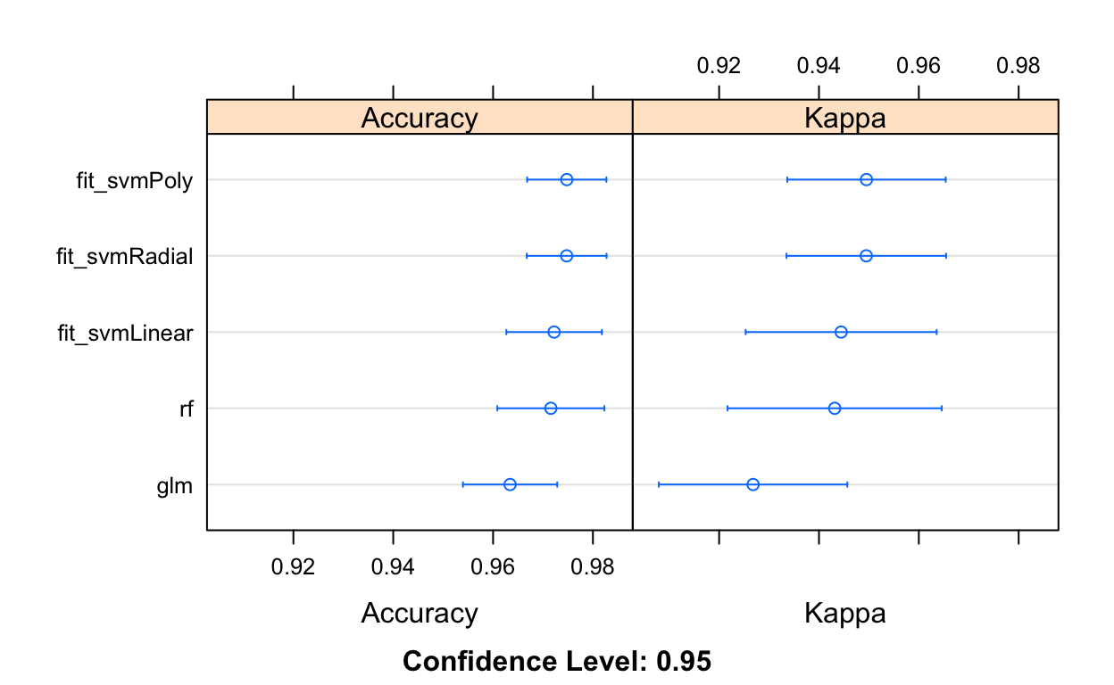
So it looks like SVM does give us a bit of a performance boost over logistic regression or random forests.
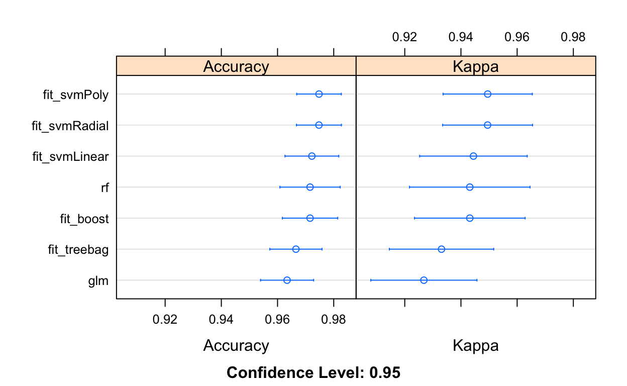
Bagging and boosting
What about bagging or boosting? Here, we try comparing existing results to both bagging and boosting (what we learned previously in class).
fit_treebag <- train(y~., data=train_dat, method="treebag",
                metric=metric, trControl=control)

fit_boost <- train(y~., data=train_dat, method="gbm",
                metric=metric, trControl=control, verbose = FALSE)
# summarize results
class_results <- resamples(list(glm=fit_glm, rf=fit_rf,
                  fit_svmLinear=fit_svmLinear, fit_svmPoly=fit_svmPoly,
                  fit_svmRadial=fit_svmRadial,
                  fit_treebag = fit_treebag,
                  fit_boost = fit_boost))
dotplot(class_results)
Checking test error rate
OK, so now that I have selected the SVM (Poly) classifier as the one that I will use (built on our train_dat), we can classify the recorded voice samples in our test_dat using the predict() function.
newdata <- as.data.frame(select(test_dat, -y))
pred_svmPoly_test <- predict(fit_svmPoly, newdata)
confusionMatrix(reference=test_dat$y, pred_svmPoly_test)
Confusion Matrix and Statistics

          Reference
Prediction   0   1
         0 778  22
         1  14 770

               Accuracy : 0.9773
                 95% CI : (0.9687, 0.984)
    No Information Rate : 0.5
    P-Value [Acc > NIR] : <2e-16

                  Kappa : 0.9545

 Mcnemar's Test P-Value : 0.2433

            Sensitivity : 0.9823
            Specificity : 0.9722
         Pos Pred Value : 0.9725
         Neg Pred Value : 0.9821
             Prevalence : 0.5000
         Detection Rate : 0.4912
   Detection Prevalence : 0.5051
      Balanced Accuracy : 0.9773

       'Positive' Class : 0