Pre-lecture materials
Read ahead
Before class, you can prepare by reading the following materials:
Acknowledgements
Material for this lecture was borrowed and adopted from
- https://rdpeng.github.io/Biostat776/lecture-literate-statistical-programming.html
- https://statsandr.com/blog/tips-and-tricks-in-rstudio-and-r-markdown/
Learning objectives
At the end of this lesson you will:
- Be able to define literate programming
- Recognize differences between available tools to for literate programming
- Know how to efficiently work within RStudio for efficient literate programming
- Create a R Markdown document
Introduction
One basic idea to make writing reproducible reports easier is what’s known as literate statistical programming (or sometimes called literate statistical practice). This comes from the idea of literate programming in the area of writing computer programs.
The idea is to think of a report or a publication as a stream of text and code. The text is readable by people and the code is readable by computers. The analysis is described in a series of text and code chunks. Each kind of code chunk will do something like load some data or compute some results. Each text chunk will relay something in a human readable language. There might also be presentation code that formats tables and figures and there’s article text that explains what’s going on around all this code. This stream of text and code is a literate statistical program or a literate statistical analysis.
Weaving and Tangling
Literate programs by themselves are a bit difficult to work with, but they can be processed in two important ways. Literate programs can be weaved to produce human readable documents like PDFs or HTML web pages, and they can tangled to produce machine-readable “documents,” or in other words, machine readable code. The basic idea behind literate programming in order to generate the different kinds of output you might need, you only need a single source document—you can weave and tangle to get the rest. In order to use a system like this you need a documentational language, that’s human readable, and you need a programming language that’s machine readable (or can be compiled/interpreted into something that’s machine readable).
Sweave
One of the original literate programming systems in R that was designed to do this was called Sweave. Sweave enables users to combine R code with a documentation program called LaTeX. Sweave files ends a .Rnw and have R code weaved through the document:
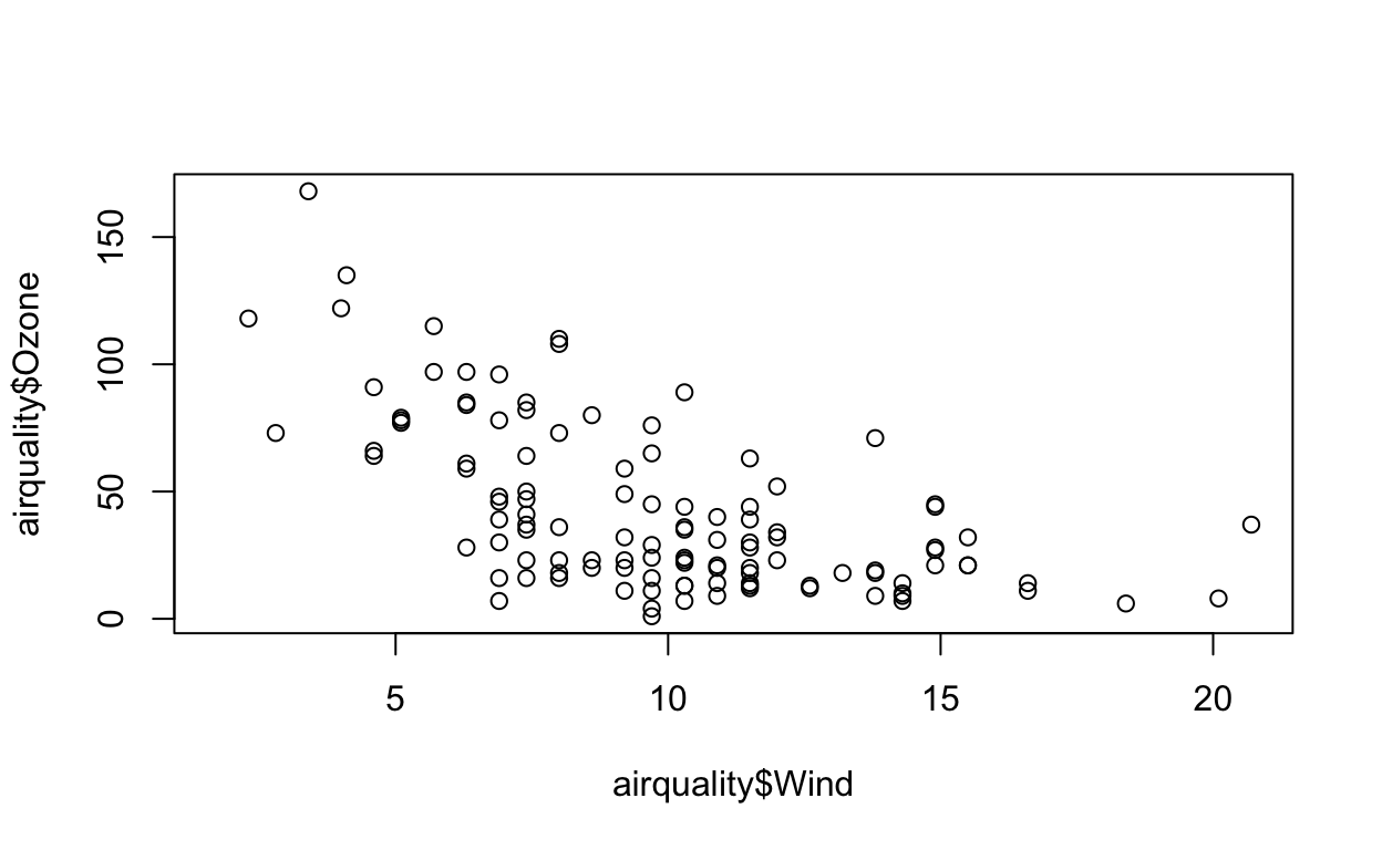
<<plot1, height=4, width=5, eval=FALSE>>=
data(airquality)
plot(airquality$Ozone ~ airquality$Wind)
@
Once you have created your .Rnw file, Sweave will process the file, executing the R chunks and replacing them with output as appropriate before creating the PDF document.
It was originally developed by Fritz Leisch, who is a core member of R, and the code base is still maintained by R Core. The Sweave system comes with any installation of R.
There are many limitations to the original Sweave system. One of the limitations is that it is focused primarily on LaTeX, which is not a documentation language that many people are familiar with. Therefore, it can be difficult to learn this type of markup language if you’re not already in a field that uses it regularly. Sweave also lacks a lot of features that people find useful like caching, and multiple plots per page and mixing programming languages.
Instead, folks have moved towards using something called knitr, which offers everything Sweave does, plus it extends it further. With Sweave, additional tools are required for advanced operations, whereas knitr supports more internally. We’ll discuss knitr below.
rmarkdown
Another choice for literate programming is to build documents based on Markdown language. A markdown file is a plain text file that is typically given the extension .md.. The rmarkdown R package takes a R Markdown file (.Rmd) and weaves together R code chunks like this:
```{r plot1, height=4, width=5, eval=FALSE, echo=TRUE}
data(airquality)
plot(airquality$Ozone ~ airquality$Wind)
```
The best resource for learning about R Markdown this by Yihui Xie, J. J. Allaire, and Garrett Grolemund:
The R Markdown Cookbook by Yihui Xie, Christophe Dervieux, and Emily Riederer is really good too:
The authors of the 2nd book describe the motivation for the 2nd book as:
“However, we have received comments from our readers and publisher that it would be beneficial to provide more practical and relatively short examples to show the interesting and useful usage of R Markdown, because it can be daunting to find out how to achieve a certain task from the aforementioned reference book (put another way, that book is too dry to read). As a result, this cookbook was born.”
Because this is lecture is built in a .Rmd file, let’s demonstrate how this work. I am going to change eval=FALSE to eval=TRUE.
- Why do we not see the back ticks ``` anymore in the code chunk above that made the plot?
- What do you think we should do if we want to have the code executed, but we want to hide the code that made it?
Before we leave this section, I find that there is quite a bit of terminology to understand the magic behind rmarkdown that can be confusing, so let’s break it down:
- Pandoc. Pandoc is a command line tool with no GUI that converts documents (e.g. from number of different markup formats to many other formats, such as .doc, .pdf etc). It is completely independent from R (but does come bundled with RStudio).
- Markdown (markup language). Markdown is a lightweight markup language with plain text formatting syntax designed so that it can be converted to HTML and many other formats. A markdown file is a plain text file that is typically given the extension
.md.It is completely independent from R. markdown(R package).markdownis an R package which converts.mdfiles into HTML. It is no longer recommended for use has been surpassed byrmarkdown(discussed below).- R Markdown (markup language). R Markdown is an extension of the markdown syntax. R Markdown files are plain text files that typically have the file extension
.Rmd. rmarkdown(R package). The R packagermarkdownis a library that uses pandoc to process and convert.Rmdfiles into a number of different formats. This core function isrmarkdown::render(). Note: this package only deals with the markdown language. If the input file is e.g..Rhtmlor.Rnw, then you need to useknitrprior to calling pandoc (see below).
Check out the R Markdown Quick Tour for more:
knitr
One of the alternative that has come up in recent times is something called knitr. The knitr package for R takes a lot of these ideas of literate programming and updates and improves upon them. knitr still uses R as its programming language, but it allows you to mix other programming languages in. You can also use a variety of documentation languages now, such as LaTeX, markdown and HTML. knitr was developed by Yihui Xie while he was a graduate student at Iowa State and it has become a very popular package for writing literate statistical programs.
Knitr takes a plain text document with embedded code, executes the code and ‘knits’ the results back into the document.
For for example, it converts
- An R Markdown (
.Rmd)file into a standard markdown file (.md) - An
.Rnw(Sweave) file into to.texformat. - An
.Rhtmlfile into to.html.
The core function is knitr::knit() and by default this will look at the input document and try and guess what type it is e.g. Rnw, Rmd etc.
This core function performs three roles:
- A source parser, which looks at the input document and detects which parts are code that the user wants to be evaluated.
- A code evaluator, which evaluates this code
- An output renderer, which writes the results of evaluation back to the document in a format which is interpretable by the raw output type. For instance, if the input file is an
.Rmd, the output render marks up the output of code evaluation in.mdformat.

Figure 1: Converting a Rmd file to many outputs using knitr and pandoc
[Source]
As seen in the figure above, from there pandoc is used to convert e.g. a .md file into many other types of file formats into a .html, etc.
So in summary:
“R Markdown stands on the shoulders of knitr and Pandoc. The former executes the computer code embedded in Markdown, and converts R Markdown to Markdown. The latter renders Markdown to the output format you want (such as PDF, HTML, Word, and so on).”
[Source]
Create and Knit Your First R Markdown Document
When creating your first R Markdown document, in RStudio you can
Go to File > New File > R Markdown…
Feel free to edit the Title
Make sure to select “Default Output Format” to be HTML
Click “OK.” RStudio creates the R Markdown document and places some boilerplate text in there just so you can see how things are setup.
Click the “Knit” button (or go to File > Knit Document) to make sure you can create the HTML output
If you successfully knit your first R Markdown document, then congratulations!

Figure 2: Mission accomplished!
Websites and Books in R Markdown
Now that you are on the road to using R Markdown documents, it is important to know about other wonderful things you do with these documents. For example, let’s say you have multiple .Rmd documents that you want to put together into a website, blog, book, etc.
There are primarily two ways to build multiple .Rmd documents together:
In this section, we briefly introduce both packages, but it’s worth mentioning that the rmarkdown package also has a built-in site generator to build websites.
blogdown
Figure 3: blogdown logo
[Source]
The blogdown R package is built on top of R Markdown, supports multi-page HTML output to write a blog post or a general page in an Rmd document, or a plain Markdown document. These source documents (e.g. .Rmd or .md) are built into a static website (i.e. a bunch of static HTML files, images and CSS files). Using this folder of files, it is very easy to publish it to any web server as a website. Also, it is easy to maintain because it is only a single folder.
For example, my personal website was built in blogdown:
Other really great examples can be found here:
Other advantages include the content likely being reproducible, easier to maintain, and easy to convert pages to e.g. PDF or other formats in the future if you do not want to convert to HTML files. Because it is based on the Markdown syntax, it is easy to write technical documents, including math equations, insert figures or tables with captions, cross-reference with figure or table numbers, add citations, and present theorems or proofs.
Here’s a video you can watch of someone making a blogdown website.
[Source on YouTube]
bookdown
Figure 4: blogdown logo
[Source]
Similar to blogdown, the bookdown R package is built on top of R Markdown, but also offers features like multi-page HTML output, numbering and cross-referencing figures/tables/sections/equations, inserting parts/appendices, and imported the GitBook style (https://www.gitbook.com) to create elegant and appealing HTML book pages. Share
For example, the previous version of this course was built in bookdown:
Another example is the Tidyverse Skills for Data Science book that the JHU Data Science Lab wrote. The github repo that contains all the .Rmd files can be found here.
Note: Even though the word “book” is in “bookdown,” this package is not only for books. It really can be anything that consists of multiple .Rmd documents meant to be read in a linear sequence such as course dissertation/thesis, handouts, study notes, a software manual, a thesis, or even a diary.
distill
There is another great way to build blogs or websites using the distill for R Markdown.
Distill for R Markdown combines the technical authoring features of the Distill web framework (optimized for scientific and technical communication) with R Markdown, enabling a fully reproducible workflow based on literate programming (Knuth 1984).
Distill articles include:
- Reader-friendly typography that adapts well to mobile devices.
- Features essential to technical writing like LaTeX math, citations, and footnotes.
- Flexible figure layout options (e.g. displaying figures at a larger width than the article text).
- Attractively rendered tables with optional support for pagination.
- Support for a wide variety of diagramming tools for illustrating concepts. The ability to incorporate JavaScript and D3-based interactive visualizations.
- A variety of ways to publish articles, including support for publishing sets of articles as a Distill website or as a Distill blog.
This course website is built in Distill for R Markdown:
- Website: https://stephaniehicks.com/jhustatcomputing2021
- Github: https://github.com/stephaniehicks/jhustatcomputing2021
Some other cool things about distill is the use of footnotes and asides.
For example.1 The number of the footnote will be automatically generated.
You can also optionally include notes in the gutter of the article (immediately to the right of the article text). To do this use the aside tag.
You can also include figures in the gutter. Just enclose the code chunk which generates the figure in an aside tag
Tips and tricks in R Markdown in RStudio
Here are shortcuts and tips on efficiently using RStudio to improve how you write code.
Run code
If you want to run a code chunk:
command + Enter on Mac
Ctrl + Enter on Windows
Insert a comment in R and R Markdown
To insert a comment:
command + Shift + C on Mac
Ctrl + Shift + C on Windows
This shortcut can be used both for:
- R code when you want to comment your code. It will add a
#at the beginning of the line - for text in R Markdown. It will add
<!--and-->around the text
Note that if you want to comment more than one line, select all the lines you want to comment then use the shortcut. If you want to uncomment a comment, apply the same shortcut.
Knit a R Markdown document
You can knit R Markdown documents by using this shortcut:
command + Shift + K on Mac
Ctrl + Shift + K on Windows
Code snippets
Code snippets is usually a few characters long and is used as a shortcut to insert a common piece of code. You simply type a few characters then press Tab and it will complete your code with a larger code. Tab is then used again to navigate through the code where customization is required. For instance, if you type fun then press Tab, it will auto-complete the code with the required code to create a function:
name <- function(variables) {

}
Pressing Tab again will jump through the placeholders for you to edit it. So you can first edit the name of the function, then the variables and finally the code inside the function (try by yourself!).
There are many code snippets by default in RStudio. Here are the code snippets I use most often:
libto calllibrary()
library(package)
matto create a matrix
matrix(data, nrow = rows, ncol = cols)
if,el, andeito create conditional expressions such asif() {},else {}andelse if () {}
if (condition) {

}

else {

}

else if (condition) {

}funto create a function
name <- function(variables) {

}
forto create for loops
for (variable in vector) {

}
tsto insert a comment with the current date and time (useful if you have very long code and share it with others so they see when it has been edited)
# Tue Jan 21 20:20:14 2020 ------------------------------
You can see all default code snippets and add yours by clicking on Tools > Global Options… > Code (left sidebar) > Edit Snippets…
Ordered list in R Markdown
In R Markdown, when creating an ordered list such as this one:
- Item 1
- Item 2
- Item 3
Instead of bothering with the numbers and typing
1. Item 1
2. Item 2
3. Item 3
you can simply type
1. Item 1
1. Item 2
1. Item 3
for the exact same result (try it yourself or check the code of this article!). This way you do not need to bother which number is next when creating a new item.
To go even further, any numeric will actually render the same result as long as the first item is the number you want to start from. For example, you could type:
1. Item 1
7. Item 2
3. Item 3
which renders
- Item 1
- Item 2
- Item 3
However, I suggest always using the number you want to start from for all items because if you move one item at the top, the list will start with this new number. For instance, if we move 7. Item 2 from the previous list at the top, the list becomes:
7. Item 2
1. Item 1
3. Item 3
which incorrectly renders
- Item 2
- Item 1
- Item 3
New code chunk in R Markdown
When editing R Markdown documents, you will need to insert a new R code chunk many times. The following shortcuts will make your life easier:
command + option + I on Mac (or command + alt + I depending on your keyboard)
Ctrl + ALT + I on Windows
Reformat code
A clear and readable code is always easier and faster to read (and look more professional when sharing it to collaborators). To automatically apply the most common coding guidelines such as white spaces, indents, etc., use:
cmd + Shift + A on Mac
Ctrl + Shift + A on Windows
So for example the following code which does not respect the guidelines (and which is not easy to read):
1+1
  for(i in 1:10){if(!i%%2){next}
print(i)
 }
becomes much more neat and readable:
1 + 1
for (i in 1:10) {
  if (!i %% 2) {
    next
  }
  print(i)
}
RStudio addins
RStudio addins are extensions which provide a simple mechanism for executing advanced R functions from within RStudio. In simpler words, when executing an addin (by clicking a button in the Addins menu), the corresponding code is executed without you having to write the code. RStudio addins have the advantage that they allow you to execute complex and advanced code much more easily than if you would have to write it yourself.
For more information about RStudio addins, check out:
Others
Similar to many other programs, you can also use:
command + Shift + Non Mac andCtrl + Shift + Non Windows to open a new R Scriptcommand + Son Mac andCtrl + Son Windows to save your current script or R Markdown document
Check out Tools –> Keyboard Shortcuts Help to see a long list of these shortcuts.
Post-lecture materials
Final Questions
Here are some post-lecture questions to help you think about the material discussed.
Questions:
What is literate programming?
What was the first literate statistical programming tool to weave together a statistical language (R) with a markup language (LaTeX)?
What is
knitrand how is different than other literate statistical programming tools?Where can you find a list of other commands that help make your code writing more efficient in RStudio?
Additional Resources
This will become a hover-able footnote↩︎