“When writing code, you’re always collaborating with future-you; and past-you doesn’t respond to emails”. —Hadley Wickham
[Source]
Pre-lecture materials
Read ahead
Before class, you can prepare by reading the following materials:
Acknowledgements
Material for this lecture was borrowed and adopted from
- https://rdpeng.github.io/Biostat776/lecture-getting-and-cleaning-data.html
- https://r4ds.had.co.nz/data-import.html
Learning objectives
At the end of this lesson you will:
- Know difference between relative vs absolute paths
- Be able to read and write text / csv files in R
- Be able to read and write R data objects in R
- Be able to calculate memory requirements for R objects
- Use modern R packages for reading and writing data
Cat meme

Figure 1: Meme: that variable should be cat-egorical
[Source]
Introduction
This lesson introduces ways to read and write data (e.g. .txt and .csv files) using base R functions as well as more modern R packages, such as readr, which is typically 10x faster than base R.
We will also briefly describe different ways for reading and writing other data types such as, Excel files, google spreadsheets, or SQL databases.
Relative versus absolute paths
When you are starting a data analysis, you have already learned about the use of .Rproj files. When you open up a .Rproj file, RStudio changes the path (location on your computer) to the .Rproj location.
After opening up a .Rproj file, you can test this by
getwd()
When you open up someone else’s R code or analysis, you might also see the
setwd()
function being used which explicitly tells R to change the absolute path or absolute location of which directory to move into.
For example, say I want to clone a GitHub repo from Roger, which has 100 R script files, and in every one of those files at the top is:
setwd("C:\Users\Roger\path\only\that\Roger\has")The problem is, if I want to use his code, I will need to go and hand-edit every single one of those paths (C:\Users\Roger\path\only\that\Roger\has) to the path that I want to use on my computer or wherever I saved the folder on my computer (e.g. /Users/Stephanie/Documents/path/only/I/have).
- This is an unsustainable practice.
- I can go in and manually edit the path, but this assumes I know how to set a working directory. Not everyone does.
So instead of absolute paths:
A better idea is to use relative paths:
Within R, an even better idea is to use the here R package will recognize the top-level directory of a Git repo and supports building all paths relative to that. For more on project-oriented workflow suggestions, read this post from Jenny Bryan.

Figure 2: Artwork by Allison Horst on on the setwd function
[Source: Artwork by Allison Horst]
The here package
In her post, Jenny Bryan writes
“I suggest organizing each data analysis into a project: a folder on your computer that holds all the files relevant to that particular piece of work.”
Instead of using setwd() at the top your .R or .Rmd file, she suggests:
- Organize each logical project into a folder on your computer.
- Make sure the top-level folder advertises itself as such. This can be as simple as having an empty file named
.here. Or, if you use RStudio and/or Git, those both leave characteristic files behind that will get the job done. - Use the
here()function from theherepackage to build the path when you read or write a file. Create paths relative to the top-level directory. - Whenever you work on this project, launch the R process from the project’s top-level directory. If you launch R from the shell,
cdto the correct folder first.
Let’s test this out. We can use getwd() to see our current working directory path and the files available using list.files()
getwd()
[1] "/Users/shicks/Documents/github/teaching/jhustatcomputing2021/_posts/2021-09-07-reading-and-writing-data"[1] "reading-and-writing-data_files" "reading-and-writing-data.html"
[3] "reading-and-writing-data.Rmd" OK so our current location is in the reading and writing lectures sub-folder of the jhustatcomputing2021 course repository. Let’s try using the here package.
library(here)

list.files(here::here())
 [1] "_custom.html"               "_exercises"
 [3] "_post_template.Rmd"         "_posts"
 [5] "_projects"                  "_projects_custom.html"
 [7] "_site.yml"                  "courses.css"
 [9] "data"                       "docs"
[11] "downloads"                  "images"
[13] "index.Rmd"                  "jhustatcomputing2021.Rproj"
[15] "lectures.Rmd"               "projects.Rmd"
[17] "README.md"                  "resources.Rmd"
[19] "schedule.Rmd"               "syllabus.Rmd"
[21] "videos" list.files(here("data"))
[1] "2016-07-19.csv.bz2" "chicago.rds" "team_standings.csv"Now we see that using the here::here() function is a relative path (relative to the .Rproj file in our jhustatcomputing2021 repository. We also see there is are two .csv files in the data folder. We will learn how to read those files into R in the next section.

Figure 3: Artwork by Allison Horst on the here package
[Source: Artwork by Allison Horst]
Finding and creating files locally
One last thing. If you want to download a file, one way to use the file.exists(), dir.create() and list.files() functions.
file.exists(here("my", "relative", "path")): logical test if the file existsdir.create(here("my", "relative", "path")): create a folderlist.files(here("my", "relative", "path")): list contents of folderfile.create(here("my", "relative", "path")): create a filefile.remove(here("my", "relative", "path")): delete a file
For example, I can put all this together by
- Checking to see if a file exists in my path. If not, then
- Create a directory in that path.
- List the files in the path.
if(!file.exists(here("my", "relative", "path"))){
  dir.create(here("my", "relative", "path"))
}
list.files(here("my", "relative", "path"))
Let’s put relative paths to use while reading and writing data.
Reading data in base R
In this section, we’re going to demonstrate the essential functions you need to know to read and write (or save) data in R.
txt or csv
There are a few primary functions reading data from base R.
read.table(),read.csv(): for reading tabular datareadLines(): for reading lines of a text file
There are analogous functions for writing data to files
write.table(): for writing tabular data to text files (i.e. CSV) or connectionswriteLines(): for writing character data line-by-line to a file or connection
Let’s try reading some data into R with the read.csv() function.
   Standing         Team
1         1        Spain
2         2  Netherlands
3         3      Germany
4         4      Uruguay
5         5    Argentina
6         6       Brazil
7         7        Ghana
8         8     Paraguay
9         9        Japan
10       10        Chile
11       11     Portugal
12       12          USA
13       13      England
14       14       Mexico
15       15  South Korea
16       16     Slovakia
17       17  Ivory Coast
18       18     Slovenia
19       19  Switzerland
20       20 South Africa
21       21    Australia
22       22  New Zealand
23       23       Serbia
24       24      Denmark
25       25       Greece
26       26        Italy
27       27      Nigeria
28       28      Algeria
29       29       France
30       30     Honduras
31       31     Cameroon
32       32  North Korea
We can use the $ symbol to pick out a specific column:
df$Team
 [1] "Spain"        "Netherlands"  "Germany"      "Uruguay"
 [5] "Argentina"    "Brazil"       "Ghana"        "Paraguay"
 [9] "Japan"        "Chile"        "Portugal"     "USA"
[13] "England"      "Mexico"       "South Korea"  "Slovakia"
[17] "Ivory Coast"  "Slovenia"     "Switzerland"  "South Africa"
[21] "Australia"    "New Zealand"  "Serbia"       "Denmark"
[25] "Greece"       "Italy"        "Nigeria"      "Algeria"
[29] "France"       "Honduras"     "Cameroon"     "North Korea"
We can also ask for the full paths for specific files
here("data", "team_standings.csv")
[1] "/Users/shicks/Documents/github/teaching/jhustatcomputing2021/data/team_standings.csv"Questions:
- What happens when you use
readLines()function with theteam_standings.csvdata? - How would you only read in the first 5 lines?
R code
Sometimes, someone will give you a file that ends in a .R. This is what’s called an R script file. It may contain code someone has written (maybe even you!), for example, a function that you can use with your data. In this case, you want the function available for you to use. To use the function, you have to first, read in the function from R script file into R.
You can check to see if the function already is loaded in R by looking at the Environment tab.
The function you want to use is
source(): for reading in R code files
For example, it might be something like this:
R objects
Alternatively, you might be interested in reading and writing R objects.
Writing data in e.g. .txt, .csv or Excel file formats is good if you want to open these files with other analysis software, such as Excel. However, these formats do not preserve data structures, such as column data types (numeric, character or factor). In order to do that, the data should be written out in a R data format.
There are several types R data file formats to be aware of:
.RData: Stores multiple R objects.Rda: This is short for.RDataand is equivalent..Rds: Stores a single R object
Question: why is saving data in as a R object useful?
Saving data into R data formats can typically reduce considerably the size of large files by compression.
Next, we will learn how to save
- A single R object
- Multiple R objects
- Your entire work space in a specified file
Reading in data from files
load(): for reading in single or multiple R objects (opposite ofsave()) with a.Rdaor.RDatafile format (objects must be same name)readRDS(): for reading in a single object with a.Rdsfile format (can rename objects)unserialize(): for reading single R objects in binary form
Writing data to files
save(): for saving an arbitrary number of R objects in binary format (possibly compressed) to a file.saveRDS(): for saving a single objectserialize(): for converting an R object into a binary format for outputting to a connection (or file).save.image(): short for ’save my current workspace; while this sounds nice, it’s not terribly useful for reproducibility (hence not suggested); it’s also what happens when you try to quit R and it asks if you want to save your work space.
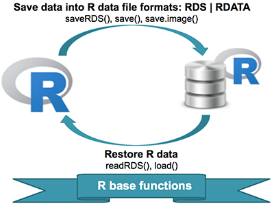
Figure 4: Save data into R data file formats: RDS and RDATA
[Source]
Let’s try an example. Let’s save a vector of length 5 into the two file formats.
x <- 1:5
save(x, file=here("data", "x.Rda"))
saveRDS(x, file=here("data", "x.Rds"))
list.files(path=here("data"))
[1] "2016-07-19.csv.bz2" "chicago.rds"        "team_standings.csv"
[4] "x.Rda"              "x.Rds"
Here we assign the imported data to an object using readRDS()
Here we assign the imported data to an object using load()
NOTE: load() simply returns the name of the objects loaded. Not the values.
Let’s clean up our space.
What do you think this code will do?
Hint: change eval=TRUE to see result
file.remove(here("data", "x.Rda"))
Now, there are of course, many R packages that have been developed to read in all kinds of other datasets, and you may need to resort to one of these packages if you are working in a specific area.
For example, check out
DBIfor relational databaseshavenfor SPSS, Stata, and SAS datahttrfor web APIsreadxlfor.xlsand.xlsxsheetsgooglesheets4for Google Sheetsgoogledrivefor Google Drive filesrvestfor web scrapingjsonlitefor JSONxml2for XML.
Reading data files with read.table()
The read.table() function is one of the most commonly used functions for reading data. The help file for read.table() is worth reading in its entirety if only because the function gets used a lot (run ?read.table in R). I know, I know, everyone always says to read the help file, but this one is actually worth reading.
The read.table() function has a few important arguments:
file, the name of a file, or a connectionheader, logical indicating if the file has a header linesep, a string indicating how the columns are separatedcolClasses, a character vector indicating the class of each column in the datasetnrows, the number of rows in the dataset. By defaultread.table()reads an entire file.comment.char, a character string indicating the comment character. This defalts to"#". If there are no commented lines in your file, it’s worth setting this to be the empty string"".skip, the number of lines to skip from the beginningstringsAsFactors, should character variables be coded as factors? This defaults toFALSE. However, back in the “old days”, it defaulted toTRUE. The reason for this was because, if you had data that were stored as strings, it was because those strings represented levels of a categorical variable. Now, we have lots of data that is text data and they do not always represent categorical variables. So you may want to set this to beFALSEin those cases. If you always want this to beFALSE, you can set a global option viaoptions(stringsAsFactors = FALSE). I’ve never seen so much heat generated on discussion forums about an R function argument than thestringsAsFactorsargument. Seriously.
For small to moderately sized datasets, you can usually call read.table() without specifying any other arguments
data <- read.table("foo.txt")
Note: foo.txt is not a real dataset here. It is only used as an example for how to use read.table().
In this case, R will automatically:
- skip lines that begin with a #
- figure out how many rows there are (and how much memory needs to be allocated)
- figure what type of variable is in each column of the table.
Telling R all these things directly makes R run faster and more efficiently. The read.csv() function is identical to read.table() except that some of the defaults are set differently (like the sep argument).
Reading in larger datasets with read.table()
With much larger datasets, there are a few things that you can do that will make your life easier and will prevent R from choking.
- Read the help page for
read.table(), which contains many hints - Make a rough calculation of the memory required to store your dataset (see the next section for an example of how to do this). If the dataset is larger than the amount of RAM on your computer, you can probably stop right here.
- Set
comment.char = ""if there are no commented lines in your file. - Use the
colClassesargument. Specifying this option instead of using the default can makeread.table()run MUCH faster, often twice as fast. In order to use this option, you have to know the class of each column in your data frame. If all of the columns are “numeric”, for example, then you can just setcolClasses = "numeric". A quick an dirty way to figure out the classes of each column is the following:
initial <- read.table("datatable.txt", nrows = 100)
classes <- sapply(initial, class)
tabAll <- read.table("datatable.txt", colClasses = classes)
Note: datatable.txt is not a real dataset here. It is only used as an example for how to use read.table().
- Set
nrows. This does not make R run faster but it helps with memory usage. A mild overestimate is okay. You can use the Unix toolwcto calculate the number of lines in a file.
In general, when using R with larger datasets, it’s also useful to know a few things about your system.
- How much memory is available on your system?
- What other applications are in use? Can you close any of them?
- Are there other users logged into the same system?
- What operating system ar you using? Some operating systems can limit the amount of memory a single process can access
Calculating Memory Requirements for R Objects
Because R stores all of its objects physical memory, it is important to be cognizant of how much memory is being used up by all of the data objects residing in your workspace. One situation where it is particularly important to understand memory requirements is when you are reading in a new dataset into R. Fortunately, it is easy to make a back of the envelope calculation of how much memory will be required by a new dataset.
For example, suppose I have a data frame with 1,500,000 rows and 120 columns, all of which are numeric data. Roughly, how much memory is required to store this data frame?
Well, on most modern computers double precision floating point numbers are stored using 64 bits of memory, or 8 bytes. Given that information, you can do the following calculation
1,500,000 × 120 × 8 bytes/numeric = 1,440,000,000 bytes
= 1,440,000,000 / 220 bytes/MB
= 1,373.29 MB
= 1.34 GB
So the dataset would require about 1.34 GB of RAM. Most computers these days have at least that much RAM. However, you need to be aware of
- what other programs might be running on your computer, using up RAM
- what other R objects might already be taking up RAM in your workspace
Reading in a large dataset for which you do not have enough RAM is one easy way to freeze up your computer (or at least your R session). This is usually an unpleasant experience that usually requires you to kill the R process, in the best case scenario, or reboot your computer, in the worst case. So make sure to do a rough calculation of memory requirements before reading in a large dataset. You’ll thank me later.
Using the readr package
The readr package is recently developed by RStudio to deal with reading in large flat files quickly. The package provides replacements for functions like read.table() and read.csv(). The analogous functions in readr are read_table() and read_csv(). These functions are often much faster than their base R analogues and provide a few other nice features such as progress meters.
For example, the package includes a variety of functions in the read_* family that allow you to read in data from different formats of flat files. The following table gives a guide to several functions in the read_* family.
readr function |
Use |
|---|---|
read_csv |
Reads comma-separated file |
read_csv2 |
Reads semicolon-separated file |
read_tsv |
Reads tab-separated file |
read_delim |
General function for reading delimited files |
read_fwf |
Reads fixed width files |
read_log |
Reads log files |
Note: In this code, I have used the kable() function from the knitr package to create the summary table in a table format, rather than as basic R output. This function is very useful for formatting basic tables in R markdown documents. For more complex tables, check out the pander and xtable packages.
For the most part, you can read use read_table() and read_csv() pretty much anywhere you might use read.table() and read.csv(). In addition, if there are non-fatal problems that occur while reading in the data, you will get a warning and the returned data frame will have some information about which rows/observations triggered the warning. This can be very helpful for “debugging” problems with your data before you get neck deep in data analysis.
The importance of the read_csv() function is perhaps better understood from an historical perspective. R’s built in read.csv() function similarly reads CSV files, but the read_csv() function in readr builds on that by removing some of the quirks and “gotchas” of read.csv() as well as dramatically optimizing the speed with which it can read data into R. The read_csv() function also adds some nice user-oriented features like a progress meter and a compact method for specifying column types.
A typical call to read_csv() will look as follows.
# A tibble: 32 × 2
   Standing Team
      <dbl> <chr>
 1        1 Spain
 2        2 Netherlands
 3        3 Germany
 4        4 Uruguay
 5        5 Argentina
 6        6 Brazil
 7        7 Ghana
 8        8 Paraguay
 9        9 Japan
10       10 Chile
# … with 22 more rows
By default, read_csv() will open a CSV file and read it in line-by-line. Similar to read.table(), you can tell the function to skip lines or which lines are comments:
read_csv("The first line of metadata
  The second line of metadata
  x,y,z
  1,2,3",
  skip = 2)
# A tibble: 1 × 3
      x     y     z
  <dbl> <dbl> <dbl>
1 1 2 3read_csv("# A comment I want to skip
x,y,z
1,2,3",
comment = "#")
# A tibble: 1 × 3
      x     y     z
  <dbl> <dbl> <dbl>
1     1     2     3
It will also (by default), read in the first few rows of the table in order to figure out the type of each column (i.e. integer, character, etc.). From the read_csv() help page:
If ‘NULL’, all column types will be imputed from the first 1000 rows on the input. This is convenient (and fast), but not robust. If the imputation fails, you’ll need to supply the correct types yourself.
You can specify the type of each column with the col_types argument.
In general, it is a good idea to specify the column types explicitly. This rules out any possible guessing errors on the part of read_csv(). Also, specifying the column types explicitly provides a useful safety check in case anything about the dataset should change without you knowing about it.
Note that the col_types argument accepts a compact representation. Here "cc" indicates that the first column is character and the second column is character (there are only two columns). Using the col_types argument is useful because often it is not easy to automatically figure out the type of a column by looking at a few rows (especially if a column has many missing values).
The read_csv() function will also read compressed files automatically. There is no need to decompress the file first or use the gzfile connection function. The following call reads a gzip-compressed CSV file containing download logs from the RStudio CRAN mirror.
Note that the warnings indicate that read_csv() may have had some difficulty identifying the type of each column. This can be solved by using the col_types argument.
# A tibble: 10 × 10
   date   time     size r_version r_arch r_os  package version country
   <chr>  <chr>   <int> <chr>     <chr>  <chr> <chr>   <chr>   <chr>
 1 2016-… 22:00… 1.89e6 3.3.0     x86_64 ming… data.t… 1.9.6   US
 2 2016-… 22:00… 4.54e4 3.3.1     x86_64 ming… assert… 0.1     US
 3 2016-… 22:00… 1.43e7 3.3.1     x86_64 ming… stringi 1.1.1   DE
 4 2016-… 22:00… 1.89e6 3.3.1     x86_64 ming… data.t… 1.9.6   US
 5 2016-… 22:00… 3.90e5 3.3.1     x86_64 ming… foreach 1.4.3   US
 6 2016-… 22:00… 4.88e4 3.3.1     x86_64 linu… tree    1.0-37  CO
 7 2016-… 22:00… 5.25e2 3.3.1     x86_64 darw… surviv… 2.39-5  US
 8 2016-… 22:00… 3.23e6 3.3.1     x86_64 ming… Rcpp    0.12.5  US
 9 2016-… 22:00… 5.56e5 3.3.1     x86_64 ming… tibble  1.1     US
10 2016-… 22:00… 1.52e5 3.3.1     x86_64 ming… magrit… 1.5     US
# … with 1 more variable: ip_id <int>
You can specify the column type in a more detailed fashion by using the various col_* functions. For example, in the log data above, the first column is actually a date, so it might make more sense to read it in as a Date object. If we wanted to just read in that first column, we could do
logdates <- read_csv(here("data", "2016-07-19.csv.bz2"),
                     col_types = cols_only(date = col_date()),
                     n_max = 10)
logdates
# A tibble: 10 × 1
   date
   <date>
 1 2016-07-19
 2 2016-07-19
 3 2016-07-19
 4 2016-07-19
 5 2016-07-19
 6 2016-07-19
 7 2016-07-19
 8 2016-07-19
 9 2016-07-19
10 2016-07-19
Now the date column is stored as a Date object which can be used for relevant date-related computations (for example, see the lubridate package).
Note: The read_csv() function has a progress option that defaults to TRUE. This options provides a nice progress meter while the CSV file is being read. However, if you are using read_csv() in a function, or perhaps embedding it in a loop, it is probably best to set progress = FALSE.
Post-lecture materials
Final Questions
Here are some post-lecture questions to help you think about the material discussed.
Questions:
What is the point of reference for using relative paths with the
here::here()function?Why was the argument
stringsAsFactors=TRUEhistorically used?What is the difference between
.Rdsand.Rdafile formats?What function in
readrwould you use to read a file where fields were separated with “|”?
Additional Resources