Pre-lecture materials
Read ahead
Before class, you can prepare by reading the following materials:
Acknowledgements
Material for this lecture was borrowed and adopted from
- https://rdpeng.github.io/Biostat776/lecture-object-oriented-programming.html
- https://adv-r.hadley.nz/oo.html
- https://www.educative.io/blog/object-oriented-programming
Learning objectives
At the end of this lesson you will:
- Recognize the primary object-oriented systems in R: S3, S4, and Reference Classes (RC).
- Understand the terminology of a class, object, method, constructor and generic.
- Be able to create a new S3, S4 or reference class with generics and methods
Introduction
Object oriented programming is one of the most successful and widespread philosophies of programming and is a cornerstone of many programming languages including Java, Ruby, Python, and C++.
At it’s core, object oriented programming (OOP) is a paradigm that is made up of classes and objects.
At a high-level, we use OOP to structure software programs into small, reusable pieces of code blueprints (i.e. classes), which are used to create instances of concrete objects.
The blueprint (or class) typically represents broad categories, e.g. bus or car that share attributes (e.g. color). The classes specify what attributes you want, but not the actual values for a particular object. However, when you create instances with objects, you are specifying the attributes (e.g. a blue car, a red car, etc).
In addition, classes can also contain functions, called methods available only to objects of that type. These functions are defined within the class and perform some action helpful to that specific type of object. For example, our car class may have a method repaint that changes the color attribute of our car. This function is only helpful to objects of type car, so we declare it within the car class thus making it a method.
OOP in R
Base R has three object oriented systems because the roots of R date back to 1976, when the idea of object orientated programming was barely four years old.
New object oriented paradigms were added to R as they were invented, so some of the ideas in R about OOP have gone stale in the years since. It is still important to understand these older systems since a huge amount of R code is written with them, and they are still useful and interesting! Long time object oriented programmers reading this book may find these old ideas refreshing.
The two older object oriented systems in R are called S3 and S4, and the modern system is called RC which stands for “reference classes.” Programmers who are already familiar with object oriented programming will feel at home using RC.
Today we are going to focus on S3 and S4, but we leave RC for you to review, if you wish.
In general, you should know and use S3 and this is also the OOP system that is most widely used in R. However, there are different R communities that prioritize other OOP systems (e.g. Bioconductor uses mostly S4).
Object Oriented Principles
Ok let’s talk about some OOP principles. The first is is the idea of a class and an object.
The world is made up of physical objects - the chair you are sitting in, the clock next to your bed, the bus you ride every day, etc. Just like the world is full of physical objects, your programs can be made of objects as well.
A class is a blueprint for an object: it describes the parts of an object, how to make an object, and what the object is able to do. If you were to think about a class for a bus (as in the public buses that roam the roads), this class would describe attributes for the bus like the number of seats on the bus, the number of windows, the color of the bus, the top speed of the bus, and the maximum distance the bus can drive on one tank of gas.
Buses, in general, can perform the same actions, and these actions are also described in the class: a bus can open and close its doors, the bus can steer, and the accelerator or the brake can be used to slow down or speed up the bus. Each of these actions can be described as a method, which is a function that is associated with a particular class.
We will be using this class in order to create individual bus objects, so we should provide a constructor, which is a method where we can specify attributes of the bus as arguments. This constructor method will then return an individual bus object with the attributes that we specified.
You could also imagine that after making the bus class you might want to make a special kind of class for a party bus. Party buses have all of the same attributes and methods as our bus class, but they also have additional attributes and methods like the number of refrigerators, window blinds that can be opened and closed, and smoke machines that can be turned on and off.
Instead of rewriting the entire bus class and then adding new attributes and methods, it is possible for the party bus class to inherit all of the attributes and methods from the bus class. In this framework of inheritance, we talk about the bus class as the super-class of the party bus, and the party bus is the sub-class of the bus. What this relationship means is that the party bus has all of the same attributes and methods as the bus class plus additional attributes and methods.
S3
Conveniently everything in R is an object. By “everything” I mean every single “thing” in R including numbers, functions, strings, data frames, lists, etc.
And while everything in R is an object, not everything is object-oriented.
This confusion arises because the base objects come from S, and were developed before anyone thought that S might need an OOP system. The tools and nomenclature evolved organically over many years without a single guiding principle.
Most of the time, the distinction between objects and object-oriented objects is not important. But here we need to get into the nitty gritty details so we will use the terms base objects and OO objects to distinguish them.
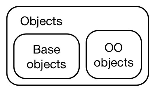
Figure 1: Everything in R is an object!
[Source]
To tell the difference between a base and OO object, use is.object()
Technically, the difference between base and OO objects is that OO objects have a “class” attribute:
This can be slightly confusing, but important to note: you can find out the class of an object in R using the class() function, but this may or may not have a class attribute.
Base types
While only OO objects have a class attribute, every object has a base type:
Base types do not form an OOP system because functions that behave differently for different base types are primarily written in C code that uses switch statements.
This means that only the R-core team can create new types, and creating a new type is a lot of work because every switch statement needs to be modified to handle a new case. As a consequence, new base types are rarely added. In total, there are 25 different base types.
Here are two more base types we have already learned about:
OO objects
At a high-level, an S3 object is a base type with at least a class attribute.
For example, take the factor. Its base type is the integer vector, it has a class attribute of “factor”, and a levels attribute that stores the possible levels:
Cool. Let’s try creating a new class in the S3 system.
In the S3 system you can arbitrarily assign a class to any object. Class assignments can be made using the structure() function, or you can assign the class using class() and <-:
As crazy as this is, it is completely legal R code, but if you want to have a better behaved S3 class you should create a constructor which returns an S3 object. The shape_S3() function below is a constructor that returns a shape_S3 object:
shape_s3 <- function(side_lengths){
  structure(list(side_lengths = side_lengths), class = "shape_S3")
}

square_4 <- shape_s3(c(4, 4, 4, 4))
class(square_4)
[1] "shape_S3"[1] "shape_S3"We have now made two shape_S3 objects: square_4 and triangle_3, which are both instantiations of the shape_S3 class.
Imagine that you wanted to create a method (or function) that would return TRUE if a shape_S3 object was a square, FALSE if a shape_S3 object was not a square, and NA if the object provided as an argument to the method was not a shape_s3 object.
This can be achieved using R’s generic methods system. A generic method can return different values based depending on the class of its input.
For example mean() is a generic method that can find the average of a vector of number or it can find the “average day” from a vector of dates. The following snippet demonstrates this behavior:
Now let’s create a generic method for identifying shape_S3 objects that are squares. The creation of every generic method uses the UseMethod() function in the following way with only slight variations:
[name of method] <- function(x) UseMethod("[name of method]")Let’s call this method is_square:
is_square <- function(x) UseMethod("is_square")
Now we can add the actual function definition for detecting whether or not a shape is a square by specifying is_square.shape_S3. By putting a dot (.) and then the name of the class after is_square, we can create a method that associates is_square with the shape_S3 class:
is_square.shape_S3 <- function(x){
  length(x$side_lengths) == 4 &&
    x$side_lengths[1] == x$side_lengths[2] &&
    x$side_lengths[2] == x$side_lengths[3] &&
    x$side_lengths[3] == x$side_lengths[4]
}

is_square(square_4)
[1] TRUEis_square(triangle_3)
[1] FALSESeems to be working well! We also want is_square() to return NA when its argument is not a shape_S3. We can specify is_square.default as a last resort if there is not method associated with the object passed to is_square().
Let’s try printing square_4:
print(square_4)
$side_lengths
[1] 4 4 4 4

attr(,"class")
[1] "shape_S3"
Doesn’t that look ugly? Lucky for us print() is a generic method, so we can specify a print method for the shape_S3 class:
print.shape_S3 <- function(x){
  if(length(x$side_lengths) == 3){
    paste("A triangle with side lengths of", x$side_lengths[1],
          x$side_lengths[2], "and", x$side_lengths[3])
  } else if(length(x$side_lengths) == 4) {
    if(is_square(x)){
      paste("A square with four sides of length", x$side_lengths[1])
    } else {
      paste("A quadrilateral with side lengths of", x$side_lengths[1],
            x$side_lengths[2], x$side_lengths[3], "and", x$side_lengths[4])
    }
  } else {
    paste("A shape with", length(x$side_lengths), "sides.")
  }
}

print(square_4)
[1] "A square with four sides of length 4"print(triangle_3)
[1] "A triangle with side lengths of 3 3 and 3"[1] "A shape with 5 sides."[1] "A quadrilateral with side lengths of 2 3 4 and 5"Since printing an object to the console is one of the most common things to do in R, nearly every class has an associated print method! To see all of the methods associated with a generic like print() use the methods() function:
 [1] "print.acf"     "print.AES"     "print.anova"   "print.aov"
 [5] "print.aovlist" "print.ar"      "print.Arima"   "print.arima0"
 [9] "print.AsIs"    "print.aspell"
One last note on S3 with regard to inheritance. In the previous section we discussed how a sub-class can inherit attributes and methods from a super-class. Since you can assign any class to an object in S3, you can specify a super class for an object the same way you would specify a class for an object:
To check if an object is a sub-class of a specified class you can use the inherits() function:
inherits(square_4, "square")
[1] TRUEExample: S3 Class/Methods for Polygons
The S3 system doesn’t have a formal way to define a class but typically, we use a list to define the class and elements of the list serve as data elements.
Here is our definition of a polygon represented using Cartesian coordinates. The class contains an element called xcoord and ycoord for the x- and y-coordinates, respectively. The make_poly() function is the “constructor” function for polygon objects. It takes as arguments a numeric vector of x-coordinates and a corresponding numeric vector of y-coordinates.
## Constructor function for polygon objects
## x a numeric vector of x coordinates
## y a numeric vector of y coordinates
make_poly <- function(x, y) {
        if(length(x) != length(y))
                stop("'x' and 'y' should be the same length")

        ## Create the "polygon" object
        object <- list(xcoord = x, ycoord = y)

        ## Set the class name
        class(object) <- "polygon"
        object
}
Now that we have a class definition, we can develop some methods for operating on objects from that class.
The first method that we will define is the print() method. The print() method should just show some simple information about the object and should not be too verbose—just enough information that the user knows what the object is.
Here the print() method just shows the user how many vertices the polygon has. It is a convention for print() methods to return the object x invisibly using the invisible() function.
Pro tip: The invisible() function is useful when it is desired to have functions return values which can be assigned, but which do not print when they are not assigned.
# These functions both return their argument

f1 <- function(x) x
f2 <- function(x) invisible(x)

f1(1)  # prints
[1] 1f2(1) # does not
However, when you assign the f2() function to an object, it does return the value
z <- f2(1)
z
[1] 1Next is the summary() method. The summary() method typically shows a bit more information and may even do some calculations. This summary() method computes the ranges of the x- and y-coordinates.
The typical approach for summary() methods is to allow the summary method to compute something, but to not print something. The strategy is
The
summary()method returns an object of class “summary_‘class name’”There is a separate
print()method for “summary_‘class name’” objects.
For example, here is the summary() method.
Note that it simply returns an object of class summary_polygon.
Now the corresponding print() method:
Now we can make use of our new class and methods.
## Construct a new "polygon" object
x <- make_poly(1:4, c(1, 5, 2, 1))
attributes(x)
$names
[1] "xcoord" "ycoord"

$class
[1] "polygon"
We can use the print() to see what the object is.
print(x)
a polygon with 4 verticesAnd we can use the summary() method to get a bit more information about the object.
Because of auto-printing we can just call the summary() method and let the results auto-print.
summary(x)
x: 1 --> 4
y: 1 --> 5 From here, we could build other methods for interacting with our polygon object. For example, it may make sense to define a plot() method or maybe methods for intersecting two polygons together.
S4
The S4 system is slightly more restrictive than S3, but it’s similar in many ways. To create a new class in S4 you need to use the setClass() function. You need to specify two or three arguments for this function: Class which is the name of the class as a string, slots, which is a named list of attributes for the class with the class of those attributes specified, and optionally contains which includes the super-class of they class you are specifying (if there is a super-class). Take look at the class definition for a bus_S4 and a party_bus_S4 below:
Now that we have created the bus_S4 and the party_bus_S4 classes we can create bus objects using the new() function. The new() function’s arguments are the name of the class and values for each “slot” in our S4 object.
my_bus <- new("bus_S4", n_seats = 20, top_speed = 80,
              current_speed = 0, brand = "Volvo")
my_bus
An object of class "bus_S4"
Slot "n_seats":
[1] 20

Slot "top_speed":
[1] 80

Slot "current_speed":
[1] 0

Slot "brand":
[1] "Volvo"
my_party_bus <- new("party_bus_S4", n_seats = 10, top_speed = 100,
current_speed = 0, brand = "Mercedes-Benz",
n_subwoofers = 2, smoke_machine_on = FALSE)
my_party_bus
An object of class "party_bus_S4"
Slot "n_subwoofers":
[1] 2

Slot "smoke_machine_on":
[1] FALSE

Slot "n_seats":
[1] 10

Slot "top_speed":
[1] 100

Slot "current_speed":
[1] 0

Slot "brand":
[1] "Mercedes-Benz"
You can use the @ operator to access the slots of an S4 object:
my_bus@n_seats
[1] 20my_party_bus@top_speed
[1] 100This is essentially the same as using the $ operator with a list or an environment.
S4 classes use a generic method system that is similar to S3 classes. In order to implement a new generic method you need to use the setGeneric() function and the standardGeneric() function in the following way:
setGeneric("new_generic", function(x){
  standardGeneric("new_generic")
})
Let’s create a generic function called is_bus_moving() to see if a bus_S4 object is in motion:
setGeneric("is_bus_moving", function(x){
  standardGeneric("is_bus_moving")
})
[1] "is_bus_moving"Now we need to actually define the function, which we can to with setMethod(). The setMethod() functions takes as arguments the name of the method as a string (or f), the method signature (signature), which specifies the class of each argument for the method, and then the function definition of the method:
setMethod(f = "is_bus_moving",
          signature = c(x = "bus_S4"),
          definition = function(x){
                          x@current_speed > 0
                      }
          )

is_bus_moving(my_bus)
[1] FALSEmy_bus@current_speed <- 1
is_bus_moving(my_bus)
[1] TRUEIn addition to creating your own generic methods, you can also create a method for your new class from an existing generic.
First, use the setGeneric() function with the name of the existing method you want to use with your class, and then use the setMethod() function like in the previous example. Let’s make a print() method for the bus_S4 class:
setGeneric("print")
[1] "print"setMethod(f = "print",
signature = c(x = "bus_S4"),
definition = function(x){
paste("This", x@brand, "bus is traveling at a speed of", x@current_speed)
})
print(my_bus)
[1] "This Volvo bus is traveling at a speed of 1"print(my_party_bus)
[1] "This Mercedes-Benz bus is traveling at a speed of 0"Reference Classes
Click here to learn about reference classes (RC).
With reference classes we leave the world of R’s old object oriented systems and enter the philosophies of other prominent object oriented programming languages. We can use the setRefClass() function to define a class’ fields, methods, and super-classes. Let’s make a reference class that represents a student:
Student <- setRefClass("Student",
                      fields = list(name = "character",
                                    grad_year = "numeric",
                                    credits = "numeric",
                                    id = "character",
                                    courses = "list"),
                      methods = list(
                        hello = function(){
                          paste("Hi! My name is", name)
                        },
                        add_credits = function(n){
                          credits <<- credits + n
                        },
                        get_email = function(){
                          paste0(id, "@jhu.edu")
                        }
                      ))
To recap: we have created a class definition called Student, which defines the student class. This class has five fields and three methods. To create a Student object use the new() method:
You can access the fields and methods of each object using the $ operator:
brooke$credits
[1] 40stephanie$hello()
[1] "Hi! My name is Stephanie"stephanie$get_email()
[1] "shicks456@jhu.edu"Methods can change the state of an object, for instance in the case of the add_credits() function:
brooke$credits
[1] 40brooke$add_credits(4)
brooke$credits
[1] 44Notice that the add_credits() method uses the complex assignment operator (<<-). You need to use this operator if you want to modify one of the fields of an object with a method. You’ll learn more about this operator in the Expressions & Environments section.
Reference classes can inherit from other classes by specifying the contains argument when they’re defined. Let’s create a sub-class of Student called Grad_Student which includes a few extra features:
Grad_Student <- setRefClass("Grad_Student",
                            contains = "Student",
                            fields = list(thesis_topic = "character"),
                            methods = list(
                              defend = function(){
                                paste0(thesis_topic, ". QED.")
                              }
                            ))

jeff <- Grad_Student$new(name = "Jeff", grad_year = 2021, credits = 8,
                    id = "jl55", courses = list("Fitbit Repair",
                                                "Advanced Base Graphics"),
                    thesis_topic = "Batch Effects")

jeff$defend()
[1] "Batch Effects. QED."Summary
- R has three object oriented systems: S3, S4, and Reference Classes.
- Reference Classes are the most similar to classes and objects in other programming languages.
- Classes are blueprints for an object.
- Objects are individual instances of a class.
- Methods are functions that are associated with a particular class.
- Constructors are methods that create objects.
- Everything in R is an object.
- S3 is a liberal object oriented system that allows you to assign a class to any object.
- S4 is a more strict object oriented system that build upon ideas in S3.
- Reference Classes are a modern object oriented system that is similar to Java, C++, Python, or Ruby.
Post-lecture materials
Additional Resources