SQL Basics

Introduction to SQL basics in R

Pre-lecture materials

Read ahead

Before class, you can prepare by reading the following materials:

1. https://dbi.r-dbi.org
2. https://db.rstudio.com/databases/sqlite/
3. https://dbplyr.tidyverse.org

Acknowledgements

Material for this lecture was borrowed and adopted from

• https://jhu-advdatasci.github.io/2019/lectures/04-gettingdata-api.html#reading_in_from_sqlite_database

Learning objectives

At the end of this lesson you will:

• Understand what are relational databases with SQL as an example
• Learn about the DBI, RSQLite, dbplyr packages for interacting with SQL databses

Before we get started, you will need to install these packages, if not already:

install.package("dbplyr") # installed with the tidyverse
install.package("RSQLite") # note: the 'DBI' package is installed here

We will also load the tidyverse for our lesson:

library(tidyverse)

Relational databases

Data live anywhere and everywhere. Data might be stored simply in a .csv or .txt file.

Data might be stored in an Excel or Google Spreadsheet. Data might be stored in large databases that require users to write special functions to interact with to extract the data they are interested in.

A relational database is a digital database based on the relational model of data, as proposed by E. F. Codd in 1970.

Figure 1: Relational model concepts

[Source: Wikipedia]

A system used to maintain relational databases is a relational database management system (RDBMS). Many relational database systems have an option of using the SQL (Structured Query Language) (or SQLite – very similar to SQL) for querying and maintaining the database.

SQL basics

Reading SQL data

There are several ways to query databases in R.

First, we will download a .sqlite database. This is a portable version of a SQL database. For our purposes, we will use the chinook sqlite database here. The database represents a “digital media store, including tables for artists, albums, media tracks, invoices and customers”.

From the Readme.md file:

Sample Data

Media related data was created using real data from an iTunes Library. … Customer and employee information was manually created using fictitious names, addresses that can be located on Google maps, and other well formatted data (phone, fax, email, etc.). Sales information is auto generated using random data for a four year period.

Here we download the data to our data folder:

library(here)
if(!file.exists(here("data", "Chinook.sqlite"))){
  file_url <- paste0("https://github.com/lerocha/chinook-database/raw/master/ChinookDatabase/DataSources/Chinook_Sqlite.sqlite")
  download.file(file_url,
                destfile=here("data", "Chinook.sqlite"))
}

We can list the files and see the .sqlite database:

list.files(here("data"))

 [1] "2016-07-19.csv.bz2"       "bmi_pm25_no2_sim.csv"    
 [3] "chicago.rds"              "Chinook.sqlite"          
 [5] "chopped.RDS"              "maacs_sim.csv"           
 [7] "nycflights13"             "storms_2004.csv.gz"      
 [9] "team_standings.csv"       "tuesdata_rainfall.RDS"   
[11] "tuesdata_temperature.RDS"

Connect to the SQL database

The main workhorse packages that we will use are the DBI and dplyr packages. Let’s look at the DBI::dbConnect() help file

?DBI::dbConnect

So we need a driver and one example is RSQLite::SQLite(). Let’s look at the help file

?RSQLite::SQLite

Ok so with RSQLite::SQLite() and DBI::dbConnect() we can connect to a SQLite database.

Let’s try that with our Chinook.sqlite file that we downloaded.

library(DBI)
conn <- DBI::dbConnect(drv = RSQLite::SQLite(), 
                       dbname = here("data", "Chinook.sqlite"))
conn

<SQLiteConnection>
  Path: /Users/shicks/Documents/github/teaching/jhustatcomputing2021/data/Chinook.sqlite
  Extensions: TRUE

So we have opened up a connection with the SQLite database. Next, we can see what tables are available in the database using the dbListTables() function:

dbListTables(conn)

 [1] "Album"         "Artist"        "Customer"      "Employee"     
 [5] "Genre"         "Invoice"       "InvoiceLine"   "MediaType"    
 [9] "Playlist"      "PlaylistTrack" "Track"        

From RStudio’s website, there are several ways to interact with SQL Databases. One of the simplest ways that we will use here is to leverage the dplyr framework.

"The dplyr package now has a generalized SQL backend for talking to databases, and the new dbplyr package translates R code into database-specific variants. As of this writing, SQL variants are supported for the following databases: Oracle, Microsoft SQL Server, PostgreSQL, Amazon Redshift, Apache Hive, and Apache Impala. More will follow over time.

So if we want to query a SQL databse with dplyr, the benefit of using dbplyr is:

"You can write your code in dplyr syntax, and dplyr will translate your code into SQL. There are several benefits to writing queries in dplyr syntax: you can keep the same consistent language both for R objects and database tables, no knowledge of SQL or the specific SQL variant is required, and you can take advantage of the fact that dplyr uses lazy evaluation.

Let’s take a closer look at the conn database that we just connected to:

library(dbplyr)
src_dbi(conn)

src:  sqlite 3.36.0 [/Users/shicks/Documents/github/teaching/jhustatcomputing2021/data/Chinook.sqlite]
tbls: Album, Artist, Customer, Employee, Genre, Invoice, InvoiceLine,
  MediaType, Playlist, PlaylistTrack, Track

You can think of the multiple tables similar to having multiple worksheets in a spreadsheet.

Let’s try interacting with one.

Querying with dplyr syntax

First, let’s look at the first ten rows in the Album table using the tbl() function from dplyr:

tbl(conn, "Album") %>%
  head(n=10)

# Source:   lazy query [?? x 3]
# Database: sqlite 3.36.0
#   [/Users/shicks/Documents/github/teaching/jhustatcomputing2021/data/Chinook.sqlite]
   AlbumId Title                                 ArtistId
     <int> <chr>                                    <int>
 1       1 For Those About To Rock We Salute You        1
 2       2 Balls to the Wall                            2
 3       3 Restless and Wild                            2
 4       4 Let There Be Rock                            1
 5       5 Big Ones                                     3
 6       6 Jagged Little Pill                           4
 7       7 Facelift                                     5
 8       8 Warner 25 Anos                               6
 9       9 Plays Metallica By Four Cellos               7
10      10 Audioslave                                   8

The output looks just like a data.frame that we are familiar with. But it’s important to know that it’s not really a dataframe. For example, what about if we use the dim() function?

tbl(conn, "Album") %>%
  dim()

[1] NA  3

Interesting! We see that the number of rows returned is NA. This is because these functions are different than operating on datasets in memory (e.g. loading data into memory using read_csv()). Instead, dplyr communicates differently with a SQLite database.

Let’s consider our example. If we were to use straight SQL, the following SQL query returns the first 10 rows from the Album table:

SELECT *
FROM `Album`
LIMIT 10

In the background, dplyr does the following:

• translates your R code into SQL
• submits it to the database
• translates the database’s response into an R data frame

To better understand the dplyr code, we can use the show_query() function:

Album <- tbl(conn, "Album")
show_query(head(Album, n = 10))

<SQL>
SELECT *
FROM `Album`
LIMIT 10

This is nice because instead of having to write the SQL query ourself, we can just use the dplyr and R syntax that we are used to.

However, the downside is that dplyr never gets to see the full Album table. It only sends our query to the database, waits for a response and returns the query. However, in this way we can interact with large datasets!

Many of the usual dplyr functions are available too:

• select()
• filter()
• summarize()

and many join functions.

Ok let’s try some of the functions out. First, let’s count how many albums each artist has made.

tbl(conn, "Album") %>%
  group_by(ArtistId) %>% 
  summarize(n = count(ArtistId)) %>% 
  head(n=10)

# Source:   lazy query [?? x 2]
# Database: sqlite 3.36.0
#   [/Users/shicks/Documents/github/teaching/jhustatcomputing2021/data/Chinook.sqlite]
   ArtistId     n
      <int> <int>
 1        1     2
 2        2     2
 3        3     1
 4        4     1
 5        5     1
 6        6     2
 7        7     1
 8        8     3
 9        9     1
10       10     1

data viz

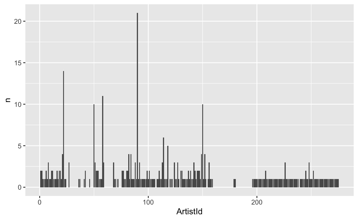
Next, let’s plot it.

tbl(conn, "Album") %>%
  group_by(ArtistId) %>% 
  summarize(n = count(ArtistId)) %>% 
  arrange(desc(n)) %>% 
  ggplot(aes(x = ArtistId, y = n)) + 
  geom_bar(stat = "identity")

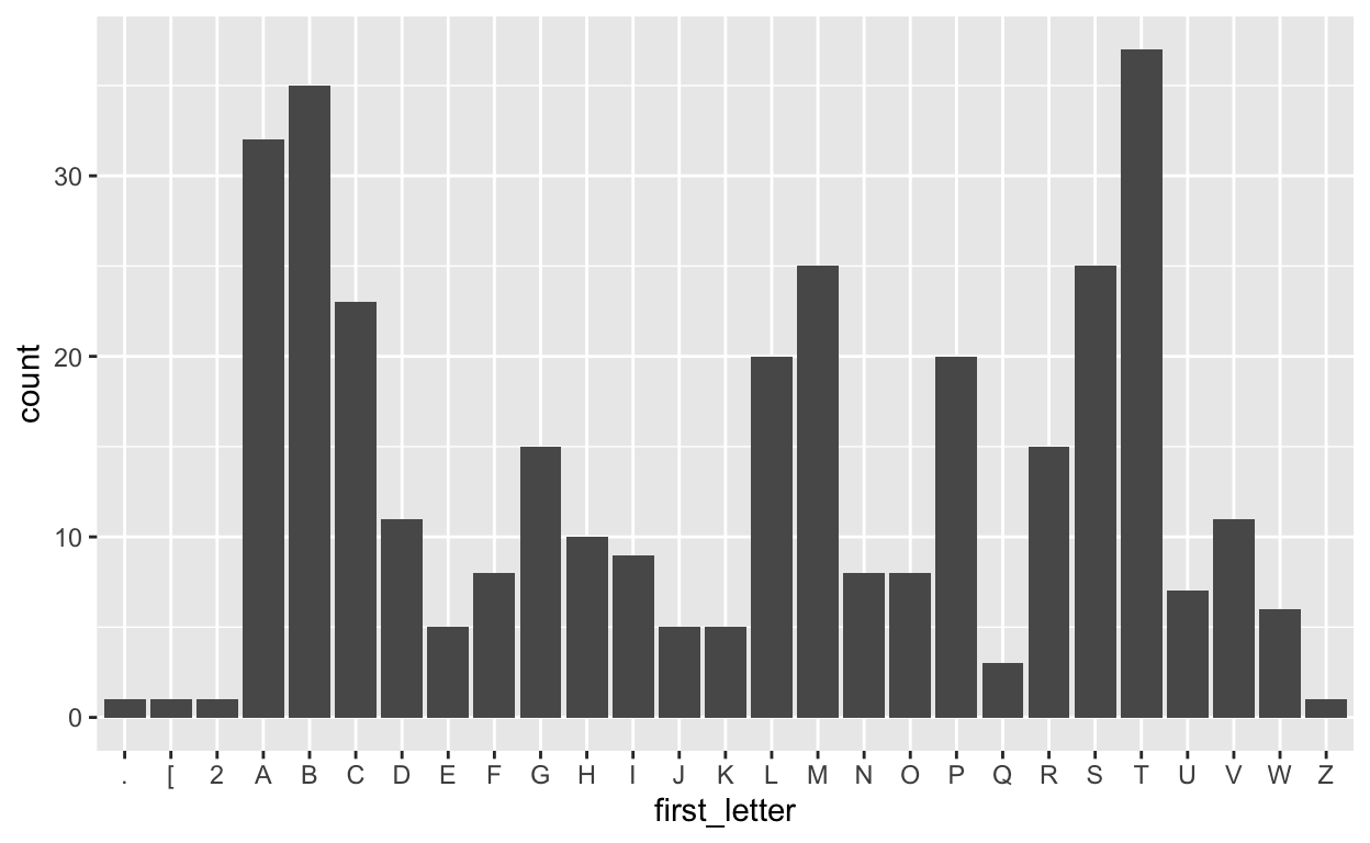
Let’s also extract the first letter from each album and plot the frequency of each letter.

tbl(conn, "Album") %>%
  mutate(first_letter = str_sub(Title, end = 1)) %>% 
  ggplot(aes(first_letter)) + 
  geom_bar()

Post-lecture materials

Additional Resources

• https://dbi.r-dbi.org
• https://db.rstudio.com/databases/sqlite/
• https://dbplyr.tidyverse.org