Project 1

Understanding songs and genres using Spotify audio features

Background

Due date: Sept 17 at 11:59pm

To submit your project

Please write up your project using R Markdown and knitr. Compile your document as an HTML file and submit your HTML file to the dropbox on Courseplus. Please show all your code for each of the answers to each part.

To get started, watch this video on setting up your R Markdown document.

Install tidyverse

Before attempting this assignment, you should first install the tidyverse package if you have not already. The tidyverse package is actually a collection of many packages that serves as a convenient way to install many packages without having to do them one by one. This can be done with the install.packages() function.

install.packages("tidyverse")

Running this function will install a host of other packages so it make take a minute or two depending on how fast your computer is. Once you have installed it, you will want to load the package.

library(tidyverse)

For all of the questions below, you can ignore the missing values in the dataset, so e.g. when taking averages, just remove the missing values before taking the average, if needed.

Data

That data for this part of the assignment comes from TidyTuesday, which is a weekly podcast and global community activity brought to you by the R4DS Online Learning Community. The goal of TidyTuesday is to help R learners learn in real-world contexts.

Figure 1: Icon from TidyTuesday

[Source: TidyTuesday]

To access the data, you need to install the tidytuesdayR R package and use the function tt_load() with the date of ‘2020-01-21’ to load the data.

install.packages("tidytuesdayR")

tuesdata <- tidytuesdayR::tt_load('2020-01-21')

    Downloading file 1 of 1: `spotify_songs.csv`

spotify_songs <- tuesdata$spotify_songs
glimpse(spotify_songs)

Rows: 32,833
Columns: 23
$ track_id                 <chr> "6f807x0ima9a1j3VPbc7VN", "0r7CVbZT…
$ track_name               <chr> "I Don't Care (with Justin Bieber) …
$ track_artist             <chr> "Ed Sheeran", "Maroon 5", "Zara Lar…
$ track_popularity         <dbl> 66, 67, 70, 60, 69, 67, 62, 69, 68,…
$ track_album_id           <chr> "2oCs0DGTsRO98Gh5ZSl2Cx", "63rPSO26…
$ track_album_name         <chr> "I Don't Care (with Justin Bieber) …
$ track_album_release_date <chr> "2019-06-14", "2019-12-13", "2019-0…
$ playlist_name            <chr> "Pop Remix", "Pop Remix", "Pop Remi…
$ playlist_id              <chr> "37i9dQZF1DXcZDD7cfEKhW", "37i9dQZF…
$ playlist_genre           <chr> "pop", "pop", "pop", "pop", "pop", …
$ playlist_subgenre        <chr> "dance pop", "dance pop", "dance po…
$ danceability             <dbl> 0.748, 0.726, 0.675, 0.718, 0.650, …
$ energy                   <dbl> 0.916, 0.815, 0.931, 0.930, 0.833, …
$ key                      <dbl> 6, 11, 1, 7, 1, 8, 5, 4, 8, 2, 6, 8…
$ loudness                 <dbl> -2.634, -4.969, -3.432, -3.778, -4.…
$ mode                     <dbl> 1, 1, 0, 1, 1, 1, 0, 0, 1, 1, 1, 1,…
$ speechiness              <dbl> 0.0583, 0.0373, 0.0742, 0.1020, 0.0…
$ acousticness             <dbl> 0.10200, 0.07240, 0.07940, 0.02870,…
$ instrumentalness         <dbl> 0.00e+00, 4.21e-03, 2.33e-05, 9.43e…
$ liveness                 <dbl> 0.0653, 0.3570, 0.1100, 0.2040, 0.0…
$ valence                  <dbl> 0.518, 0.693, 0.613, 0.277, 0.725, …
$ tempo                    <dbl> 122.036, 99.972, 124.008, 121.956, …
$ duration_ms              <dbl> 194754, 162600, 176616, 169093, 189…

If we look at the TidyTuesday github repo from 2020, we see this dataset contains songs from Spotify.

Here is a data dictionary for what all the column names mean:

• https://github.com/rfordatascience/tidytuesday/blob/master/data/2020/2020-01-21/readme.md#data-dictionary

Part 1: Explore data

In this part, use functions from dplyr to answer the following questions.

1. How many songs are in each genre?

# Add your solution here

2. What is average value of energy and acousticness in the latin genre in this dataset?

# Add your solution here

3. Calculate the average duration of song (in minutes) across all subgenres. Which subgenre has the longest song on average?

# Add your solution here

4. Make two boxplots side-by-side of the danceability of songs stratifying by whether a song has a fast or slow tempo. Define fast tempo as any song that has a tempo above its median value. On average, which songs are more danceable?

Hint: You may find the case_when() function useful in this part, which can be used to map values from one variable to different values in a new variable (when used in a mutate() call).

## Generate some random numbers
dat <- tibble(x = rnorm(100))
slice(dat, 1:3)

# A tibble: 3 × 1
       x
   <dbl>
1 0.288 
2 0.102 
3 0.0931

## Create a new column that indicates whether the value of 'x' is positive or negative
dat %>%
        mutate(is_positive = case_when(
                x >= 0 ~ "Yes",
                x < 0 ~ "No"
        ))

# A tibble: 100 × 2
         x is_positive
     <dbl> <chr>      
 1  0.288  Yes        
 2  0.102  Yes        
 3  0.0931 Yes        
 4  0.742  Yes        
 5  0.339  Yes        
 6  0.624  Yes        
 7 -0.0439 No         
 8  2.44   Yes        
 9 -1.34   No         
10 -1.85   No         
# … with 90 more rows

# Add your solution here

Part 2: Convert nontidy data into tidy data

The goal of this part of the assignment is to take a dataset that is either messy or simply not tidy and to make them tidy datasets. The objective is to gain some familiarity with the functions in the dplyr, tidyr packages. You may find it helpful to review the section on spreading and gathering data.

Tasks

This dataset gives a set of 12 audio features (e.g. acousticness, liveness, speechiness, etc) and descriptors like duration, tempo, key, and mode for a set of 32833 songs (in addition to the artist, album name, album release date, etc).

spotify_songs

# A tibble: 32,833 × 23
   track_id  track_name   track_artist track_popularity track_album_id
   <chr>     <chr>        <chr>                   <dbl> <chr>         
 1 6f807x0i… I Don't Car… Ed Sheeran                 66 2oCs0DGTsRO98…
 2 0r7CVbZT… Memories - … Maroon 5                   67 63rPSO264uRjW…
 3 1z1Hg7Vb… All the Tim… Zara Larsson               70 1HoSmj2eLcsrR…
 4 75Fpbthr… Call You Mi… The Chainsm…               60 1nqYsOef1yKKu…
 5 1e8PAfcK… Someone You… Lewis Capal…               69 7m7vv9wlQ4i0L…
 6 7fvUMiya… Beautiful P… Ed Sheeran                 67 2yiy9cd2QktrN…
 7 2OAylPUD… Never Reall… Katy Perry                 62 7INHYSeusaFly…
 8 6b1RNvAc… Post Malone… Sam Feldt                  69 6703SRPsLkS4b…
 9 7bF6tCO3… Tough Love … Avicii                     68 7CvAfGvq4RlIw…
10 1IXGILkP… If I Can't … Shawn Mendes               67 4QxzbfSsVryEQ…
# … with 32,823 more rows, and 18 more variables:
#   track_album_name <chr>, track_album_release_date <chr>,
#   playlist_name <chr>, playlist_id <chr>, playlist_genre <chr>,
#   playlist_subgenre <chr>, danceability <dbl>, energy <dbl>,
#   key <dbl>, loudness <dbl>, mode <dbl>, speechiness <dbl>,
#   acousticness <dbl>, instrumentalness <dbl>, liveness <dbl>,
#   valence <dbl>, tempo <dbl>, duration_ms <dbl>

Use the functions in dplyr, tidyr, and lubridate to perform the following steps to the spotify_songs dataset:

1. Select only unique distinct rows from the dataset based on the track_name and track_artist columns (Hint check out the distinct() function in dplyr).
2. Add a new column called year_released listing just the year that the song was released. (Hint check out the ymd() function in lubridate R package. Also, if you get a warning message with “failed to parse”, check out the truncated argument in the ymd() function.).
3. Keep only songs that were released in or after 1980.
4. Add a new column with the duration of the song in minutes
5. For each year_released, calculate the mean of at least 6 of the audio features (e.g. danceability, energy, loudness, etc), or descriptors (e.g. tempo, duration in minutes, etc). (Hint: If all has gone well thus far, you should have a dataset with 41 rows and 7 columns).
6. Convert this wide dataset into a long dataset with a new feature and mean_score column

It should look something like this:

year_released   feature   mean_score
<dbl>           <chr>       <dbl>
1980    Danceability    0.5633676       
1980    Energy  0.7107647       
1980    Loudness    -8.5211765      
1980    Valence 0.6333235       
1980    Tempo   124.1458529     
1980    Duration    4.2853662       
1981    Danceability    0.5697258       
1981    Energy  0.6967581       
1981    Loudness    -8.8678065      
1981    Valence 0.6650968   

Notes

• You may need to use functions outside these packages to obtain this result.

• Note that the functions in the dplyr and tidyr package expect table-like objects (data frames or tibbles) as their input. You can convert data to these objects using the as_tibble() function in the tibble package.

• Do not worry about the ordering of the rows or columns. Depending on whether you use gather() or pivot_longer(), the order of your output may differ from what is printed above. As long as the result is a tidy data set, that is sufficient.

# Add your solution here

Part 3: Data visualization

In this part of the project, we will continue to work with our now tidy song dataset from the previous part.

Tasks

Use the functions in ggplot2 package to make a scatter plot of the six (or more) mean_scores (y-axis) over time (x-axis). For full credit, your plot should include:

1. An overall title for the plot and a subtitle summarizing key trends that you found. Also include a caption in the figure with your name.
2. Both the observed points for the mean_score, but also a smoothed non-linear pattern of the trend
3. All six (or more) plots should be shown in the one figure
4. There should be an informative x-axis and y-axis label

Consider playing around with the theme() function to make the figure shine, including playing with background colors, font, etc.

Notes

• You may need to use functions outside these packages to obtain this result.

• Note that the functions in the dplyr and tidyr package expect table-like objects (data frames or tibbles) as their input. You can convert data to these objects using the as_tibble() function in the tibble package.

• Don’t worry about the ordering of the rows or columns. Depending on whether you use gather() or pivot_longer(), the order of your output may differ from what is printed above. As long as the result is a tidy data set, that is sufficient.

# Add your solution here

Part 4: Make the worst plot you can!

This sounds a bit crazy I know, but I want this to be FUN! Instead of trying to make a “good” plot, I want you to explore your creative side and make a really awful data visualization in every way. :)

Tasks

Using the spotify_songs dataset (and it does not have to be the tidy dataset that we created in Part 2, it can be anything from the original dataset):

1. Make the absolute worst plot that you can. You need to customize it in at least 7 ways to make it awful.
2. In your document, write 1 - 2 sentences about each different customization you added (using bullets – i.e. there should be at least 7 bullet points each with 1-2 sentences), and how it could be useful for you when you want to make an awesome data visualization.

# Add your solution here

Part 5: Make my plot a better plot!

The goal is to take my sad looking plot and make it better! If you’d like an example, here is a tweet I came across of someone who gave a talk about how to zhoosh up your ggplots.

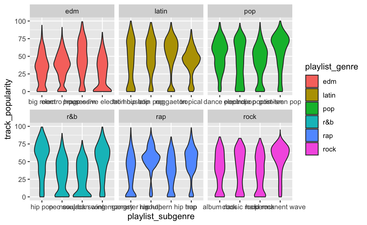
spotify_songs %>% 
  ggplot(aes(y=track_popularity, x=playlist_subgenre, fill = playlist_genre)) + 
  geom_violin() +
  facet_wrap( ~ playlist_genre, scales = "free_x")

Tasks

1. You need to customize it in at least 7 ways to make it better.
2. In your document, write 1 - 2 sentences about each different customization you added (using bullets – i.e. there should be at least 7 bullet points each with 1-2 sentences), describing how you improved it.

# Add your solution here