Pre-lecture materials

Read ahead

Before class, you can prepare by reading the following materials:

Acknowledgements

Material for this lecture was borrowed and adopted from

Learning objectives

At the end of this lesson you will:

Be able to define relational data and keys
Be able to define the three types of join functions for relational data
Be able to implement mutational join functions

Relational data

Data analyses rarely involve only a single table of data.

Typically you have many tables of data, and you must combine the datasets to answer the questions that you are interested in.

Collectively, multiple tables of data are called relational data because it is the relations, not just the individual datasets, that are important.

Relations are always defined between a pair of tables. All other relations are built up from this simple idea: the relations of three or more tables are always a property of the relations between each pair.

Sometimes both elements of a pair can be the same table! This is needed if, for example, you have a table of people, and each person has a reference to their parents.

To work with relational data you need verbs that work with pairs of tables.

Three important families of verbs

There are three families of verbs designed to work with relational data:

Mutating joins: A mutating join allows you to combine variables from two tables. It first matches observations by their keys, then copies across variables from one table to the other on the right side of the table (similar to mutate()). We will discuss a few of these below.
- See Section 4 for Table of mutating joins.
Filtering joins: Filtering joins match observations in the same way as mutating joins, but affect the observations, not the variables (i.e. filter observations from one data frame based on whether or not they match an observation in the other).
- Two types: semi_join(x, y) and anti_join(x, y).
Set operations: Treat observations as if they were set elements. Typically used less frequently, but occasionally useful when you want to break a single complex filter into simpler pieces. All these operations work with a complete row, comparing the values of every variable. These expect the x and y inputs to have the same variables, and treat the observations like sets:
- Examples of set operations: intersect(x, y), union(x, y), and setdiff(x, y).

Keys

The variables used to connect each pair of tables are called keys. A key is a variable (or set of variables) that uniquely identifies an observation. In simple cases, a single variable is sufficient to identify an observation.

Note

There are two types of keys:

A primary key uniquely identifies an observation in its own table.
A foreign key uniquely identifies an observation in another table.

Let’s consider an example to help us understand the difference between a primary key and foreign key.

Example of keys

Imagine you are conduct a study and collecting data on subjects and a health outcome.

Often, subjects will make multiple visits (a so-called longitudinal study) and so we will record the outcome for each visit. Similarly, we may record other information about them, such as the kind of housing they live in.

The first table

This code creates a simple table with some made up data about some hypothetical subjects’ outcomes.

library(tidyverse)

outcomes <- tibble(
        id = rep(c("a", "b", "c"), each = 3),
        visit = rep(0:2, 3),
        outcome = rnorm(3 * 3, 3)
)

print(outcomes)

# A tibble: 9 × 3
  id    visit outcome
  <chr> <int>   <dbl>
1 a         0   3.74 
2 a         1   4.36 
3 a         2   3.23 
4 b         0   3.22 
5 b         1   0.290
6 b         2   1.33 
7 c         0   3.14 
8 c         1   3.29 
9 c         2   3.39

Note that subjects are labeled by a unique identifer in the id column.

A second table

Here is some code to create a second table (we will be joining the first and second tables shortly). This table contains some data about the hypothetical subjects’ housing situation by recording the type of house they live in.

subjects <- tibble(
        id = c("a", "b", "c"),
        house = c("detached", "rowhouse", "rowhouse")
)

print(subjects)

# A tibble: 3 × 2
  id    house   
  <chr> <chr>   
1 a     detached
2 b     rowhouse
3 c     rowhouse

Question

What is the primary key and foreign key?

The outcomes$id is a primary key because it uniquely identifies each subject in the outcomes table.
The subjects$id is a foreign key because it appears in the subjects table where it matches each subject to a unique id.

Mutating joins

The dplyr package provides a set of functions for joining two data frames into a single data frame based on a set of key columns.

There are several functions in the *_join() family.

These functions all merge together two data frames
They differ in how they handle observations that exist in one but not both data frames.

Here, are the four functions from this family that you will likely use the most often:

Function	What it includes in merged data frame
`left_join()`	Includes all observations in the left data frame, whether or not there is a match in the right data frame
`right_join()`	Includes all observations in the right data frame, whether or not there is a match in the left data frame
`inner_join()`	Includes only observations that are in both data frames
`full_join()`	Includes all observations from both data frames

[Source from R for Data Science]

Left Join

Recall the outcomes and subjects datasets above.

outcomes

# A tibble: 9 × 3
  id    visit outcome
  <chr> <int>   <dbl>
1 a         0   3.74 
2 a         1   4.36 
3 a         2   3.23 
4 b         0   3.22 
5 b         1   0.290
6 b         2   1.33 
7 c         0   3.14 
8 c         1   3.29 
9 c         2   3.39

subjects

# A tibble: 3 × 2
  id    house   
  <chr> <chr>   
1 a     detached
2 b     rowhouse
3 c     rowhouse

Suppose we want to create a table that combines the information about houses (subjects) with the information about the outcomes (outcomes).

We can use the left_join() function to merge the outcomes and subjects tables and produce the output above.

left_join(x = outcomes, y = subjects, by = "id")

# A tibble: 9 × 4
  id    visit outcome house   
  <chr> <int>   <dbl> <chr>   
1 a         0   3.74  detached
2 a         1   4.36  detached
3 a         2   3.23  detached
4 b         0   3.22  rowhouse
5 b         1   0.290 rowhouse
6 b         2   1.33  rowhouse
7 c         0   3.14  rowhouse
8 c         1   3.29  rowhouse
9 c         2   3.39  rowhouse

Note

The by argument indicates the column (or columns) that the two tables have in common.

Left Join with Incomplete Data

In the previous examples, the subjects table didn’t have a visit column. But suppose it did? Maybe people move around during the study. We could image a table like this one.

subjects <- tibble(
        id = c("a", "b", "c"),
        visit = c(0, 1, 0),
        house = c("detached", "rowhouse", "rowhouse"),
)

print(subjects)

# A tibble: 3 × 3
  id    visit house   
  <chr> <dbl> <chr>   
1 a         0 detached
2 b         1 rowhouse
3 c         0 rowhouse

When we left joint the tables now we get:

left_join(outcomes, subjects, by = c("id", "visit"))

# A tibble: 9 × 4
  id    visit outcome house   
  <chr> <dbl>   <dbl> <chr>   
1 a         0   3.74  detached
2 a         1   4.36  <NA>    
3 a         2   3.23  <NA>    
4 b         0   3.22  <NA>    
5 b         1   0.290 rowhouse
6 b         2   1.33  <NA>    
7 c         0   3.14  rowhouse
8 c         1   3.29  <NA>    
9 c         2   3.39  <NA>

Note

Two things to point out here:

If we do not have information about a subject’s housing in a given visit, the left_join() function automatically inserts an NA value to indicate that it is missing.
We can “join” on multiple variable (e.g. here we joined on the id and the visit columns).

We may even have a situation where we are missing housing data for a subject completely. The following table has no information about subject a.

subjects <- tibble(
        id = c("b", "c"),
        visit = c(1, 0),
        house = c("rowhouse", "rowhouse"),
)

subjects

# A tibble: 2 × 3
  id    visit house   
  <chr> <dbl> <chr>   
1 b         1 rowhouse
2 c         0 rowhouse

But we can still join the tables together and the house values for subject a will all be NA.

left_join(x = outcomes, y = subjects, by = c("id", "visit"))

# A tibble: 9 × 4
  id    visit outcome house   
  <chr> <dbl>   <dbl> <chr>   
1 a         0   3.74  <NA>    
2 a         1   4.36  <NA>    
3 a         2   3.23  <NA>    
4 b         0   3.22  <NA>    
5 b         1   0.290 rowhouse
6 b         2   1.33  <NA>    
7 c         0   3.14  rowhouse
8 c         1   3.29  <NA>    
9 c         2   3.39  <NA>

Important

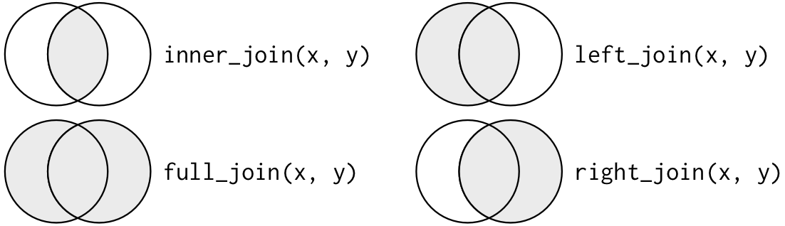
The bottom line for left_join() is that it always retains the values in the “left” argument (in this case the outcomes table).

If there are no corresponding values in the “right” argument, NA values will be filled in.

Inner Join

The inner_join() function only retains the rows of both tables that have corresponding values. Here we can see the difference.

inner_join(x = outcomes, y = subjects, by = c("id", "visit"))

# A tibble: 2 × 4
  id    visit outcome house   
  <chr> <dbl>   <dbl> <chr>   
1 b         1   0.290 rowhouse
2 c         0   3.14  rowhouse

Right Join

The right_join() function is like the left_join() function except that it gives priority to the “right” hand argument.

right_join(x = outcomes, y = subjects, by = c("id", "visit"))

# A tibble: 2 × 4
  id    visit outcome house   
  <chr> <dbl>   <dbl> <chr>   
1 b         1   0.290 rowhouse
2 c         0   3.14  rowhouse

Summary

left_join() is useful for merging a “large” data frame with a “smaller” one while retaining all the rows of the “large” data frame
inner_join() gives you the intersection of the rows between two data frames
right_join() is like left_join() with the arguments reversed (likely only useful at the end of a pipeline)

Post-lecture materials

Final Questions

Here are some post-lecture questions to help you think about the material discussed.

Questions

If you had three data frames to combine with a shared key, how would you join them using the verbs you now know?
Using df1 and df2 below, what is the difference between inner_join(df1, df2), semi_join(df1, df2) and anti_join(df1, df2)?

# Create first example data frame
df1 <- data.frame(ID = 1:3,
                  X1 = c("a1", "a2", "a3"))
# Create second example data frame
df2 <- data.frame(ID = 2:4, 
                  X2 = c("b1", "b2", "b3"))

Try changing the order from the above e.g. inner_join(df2, df1), semi_join(df2, df1) and anti_join(df2, df1). What changed? What did not change?

Additional Resources

Tip