Pre-lecture materials

Read ahead

Before class, you can prepare by reading the following materials:

Acknowledgements

Material for this lecture was borrowed and adopted from

Learning objectives

At the end of this lesson you will be able to:

Explain the difference between a table, a record, and a field in relational databases
Explain the difference between a database and a database manager
Write a query to select all values for specific fields from a single table
Write queries that display results in a particular order
Write queries that eliminate duplicate values from data
Write queries that select records that satisfy user-specified conditions
Learn about the DBI, RSQLite, dbplyr packages for making SQL queries in R

Installation

Command-line tool `sqlite3`

For this lecture, we will use Unix shell, plus SQLite3 or DB Browser for SQLite.

You can see if the command-line tool sqlite3 (also known as “SQLite”) is already installed with

sqlite3 --version

3.39.4 2022-09-07 20:51:41 6bf7a2712125fdc4d559618e3fa3b4944f5a0d8f8a4ae21165610e153f77aapl

If not, you can install with homebrew or follow the instructions here:

https://swcarpentry.github.io/sql-novice-survey/setup.html

R packages

You will need to install these R packages:

install.packages("DBI")
install.packages("RSQLite")
install.packages("dbplyr")

We will load them here before kicking off the lecture.

library(tidyverse)
library(DBI)
library(RSQLite)
library(dbplyr)

Relational databases

Data live anywhere and everywhere. Data might be stored simply in a .csv or .txt file.

Data might be stored in an Excel or Google Spreadsheet. Data might be stored in large databases that require users to write special functions to interact with to extract the data they are interested in.

A relational database is a digital database based on the relational model of data, as proposed by E. F. Codd in 1970.

Broadly relational databases are a way to store and manipulate information.

Databases are arranged as tables with a unique relation variable name
Each table has columns (also known as fields or attributes) that describe the data
Rows (also known as records) contain the data

[Source: Wikipedia]

Database managers

When we are using a spreadsheet, we put formulas into cells to calculate new values based on old ones.

When we are using a database, we send commands (usually called queries) to a database manager (a program that manipulates the database for us).

The database manager does whatever lookups and calculations the query specifies, returning the results in a tabular form that we can then use as a starting point for further queries.

Examples of database manager include:

Oracle
IBM DB2
PostgreSQL
MySQL
Microsoft Access
SQLite (which is what we will use here)

A system used to maintain relational databases is a relational database management system (RDBMS).

Languages

We write queries in a language called Structured Query Language (SQL), which provides hundreds of different ways to analyze and recombine data.

Many database managers understand SQL but each stores data in a different way, so a database created with one cannot be used directly by another.

However, every database manager can import and export data in a variety of formats like .csv, .sql, so it is possible to move information from one to another.

Next, we will some example SQL queries that are common tasks for data scientists.

SQL basics

In this next few sections, we will use the SQLite database manager and interact with it interactively on the command-line with the command sqlite3.

Getting Into and Out Of SQLite

In order to use the SQLite commands interactively, we need to enter into the SQLite console. So, open up a terminal, and run

Bash

cd data
sqlite3 survey.db

The SQLite command is sqlite3 and you are telling SQLite to open up the survey.db. You need to specify the .db file, otherwise SQLite will open up a temporary, empty database.

All SQLite-specific commands are prefixed with a . to distinguish them from SQL commands.
To get out of SQLite, type out .exit or .quit. For some terminals, Ctrl-D can also work.
If you forget any SQLite . (dot) command, type .help.

Example data

Before we get into using SQLite to select the data, let’s take a look at the tables of the database we will use in our examples:

Person: People who took readings, id being the unique identifier for that person.

id	personal	family
dyer	William	Dyer
pb	Frank	Pabodie
lake	Anderson	Lake
roe	Valentina	Roerich
danforth	Frank	Danforth

Site: Locations of the sites where readings were taken.

name	lat	long
DR-1	-49.85	-128.57
DR-3	-47.15	-126.72
MSK-4	-48.87	-123.4

Visited: Specific identification id of the precise locations where readings were taken at the sites and dates.

id	site	dated
619	DR-1	1927-02-08
622	DR-1	1927-02-10
734	DR-3	1930-01-07
735	DR-3	1930-01-12
751	DR-3	1930-02-26
752	DR-3	-null-
837	MSK-4	1932-01-14
844	DR-1	1932-03-22

Survey: The measurements taken at each precise location on these sites. They are identified as taken. The field quant is short for quantity and indicates what is being measured. The values are rad, sal, and temp referring to ‘radiation’, ‘salinity’ and ‘temperature’, respectively.

taken	person	quant	reading
619	dyer	rad	9.82
619	dyer	sal	0.13
622	dyer	rad	7.8
622	dyer	sal	0.09
734	pb	rad	8.41
734	lake	sal	0.05
734	pb	temp	-21.5
735	pb	rad	7.22
735	-null-	sal	0.06
735	-null-	temp	-26.0
751	pb	rad	4.35
751	pb	temp	-18.5
751	lake	sal	0.1
752	lake	rad	2.19
752	lake	sal	0.09
752	lake	temp	-16.0
752	roe	sal	41.6
837	lake	rad	1.46
837	lake	sal	0.21
837	roe	sal	22.5
844	roe	rad	11.25

SQL `.tables` and `.schema`

In an interactive sqlite3 session,

Type .tables to list the tables in the database
Type .schema to see the SQL statements used to create the tables in the database. The statements will have a list of the columns and the data types each column stores.

More about .schema

The output from .schema is formatted as <columnName dataType>.

Output

CREATE TABLE Person (id text, personal text, family text);
CREATE TABLE Site (name text, lat real, long real);
CREATE TABLE Survey (taken integer, person text, quant text, reading real);
CREATE TABLE Visited (id integer, site text, dated text);

Thus we can see from the first line that the table Person has three columns:

id with type text
personal with type text
family with type text

The available data types vary based on the database manager - you can search online for what data types are supported.

SQL command `SELECT`

For now, let’s write an SQL query that displays scientists’ names.

We do this using the SQL command SELECT, giving it the names of the columns we want and the table we want them from.

Our query looks like this:

SQL

SELECT family, personal FROM Person;

And the output looks like this:

Output

|family  |personal |
|--------|---------|
|Dyer    |William  |
|Pabodie |Frank    |
|Lake    |Anderson |
|Roerich |Valentina|
|Danforth|Frank    |

Important

The semicolon at the end of the query tells the database manager that the query is complete and ready to run.

We have written our commands in upper case and the names for the table and columns in lower case, but we don’t have to because SQL is case insensitive.

SQL

SeLeCt FaMiLy, PeRsOnAl FrOm PeRsOn;

Output:

Output

|family  |personal |
|--------|---------|
|Dyer    |William  |
|Pabodie |Frank    |
|Lake    |Anderson |
|Roerich |Valentina|
|Danforth|Frank    |

Pro-tip

You can use SQL’s case insensitivity to distinguish between different parts of an SQL statement.

Here, we use the convention of using

UPPER CASE for SQL keywords (such as SELECT and FROM)
Title Case for table names
lower case for field names

Whatever casing convention you choose, please be consistent: complex queries are hard enough to read without the extra cognitive load of random capitalization.

More about the ;

While we are on the topic of SQL’s syntax, one aspect of SQL’s syntax that can frustrate novices and experts alike is forgetting to finish a command with ; (semicolon).

When you press enter for a command without adding the ; to the end, it can look something like this:

Output

SELECT id FROM Person
...>
...>

This is SQL’s prompt, where it is waiting for additional commands or for a ; to let SQL know to finish.

This is easy to fix! Just type ; and press enter!

More about `SELECT`

Row and columns in a database table are not actually stored in any particular order.

They will always be displayed in some order, but we can control that in various ways.

Example

We could swap the columns in the output by writing our query as:

SQL

SELECT personal, family FROM Person;

Output

|personal |family  |
|---------|--------|
|William  |Dyer    |
|Frank    |Pabodie |
|Anderson |Lake    |
|Valentina|Roerich |
|Frank    |Danforth|

or even repeat columns:

SQL

SELECT id, id, id FROM Person;

Output

|id      |id      |id      |
|--------|--------|--------|
|dyer    |dyer    |dyer    |
|pb      |pb      |pb      |
|lake    |lake    |lake    |
|roe     |roe     |roe     |
|danforth|danforth|danforth|

The `*` operator

As a shortcut, we can select all of the columns in a table using *:

SQL

SELECT * FROM Person;

Output

|id      |personal |family  |
|--------|---------|--------|
|dyer    |William  |Dyer    |
|pb      |Frank    |Pabodie |
|lake    |Anderson |Lake    |
|roe     |Valentina|Roerich |
|danforth|Frank    |Danforth|

Sorting and removing duplicates

In this section, we will explore the following questions of the Antarctic data

What are the unique types of measurements taken in Survey?
Which scientists took measurements on the expedition?

To answer the first question, we will extract the values in column quant (short for quantity) from Survey, which contains values rad, sal, and temp referring to ‘radiation’, ‘salinity’ and ‘temperature’, respectively.

However, we only want the unique value labels.

The following will extract the quant column from the Survey table, but not return unique / distinct labels.

SQL

SELECT quant FROM Survey;

But, adding the DISTINCT keyword to our query eliminates the redundant output to make the result more readable:

SQL

SELECT DISTINCT quant FROM Survey;

Output

|quant|
|-----|
|rad  |
|sal  |
|temp |

You can also use the DISTINCT keyword on multiple columns.

If we select more than one column, distinct sets of values are returned (in this case pairs, because we are selecting two columns) and duplicates are removed:

SQL

SELECT DISTINCT taken, quant FROM Survey;

Output

|taken|quant|
|-----|-----|
|619  |rad  |
|619  |sal  |
|622  |rad  |
|622  |sal  |
|734  |rad  |
|734  |sal  |
|734  |temp |
|735  |rad  |
|735  |sal  |
|735  |temp |
|751  |rad  |
|751  |temp |
|751  |sal  |
|752  |rad  |
|752  |sal  |
|752  |temp |
|837  |rad  |
|837  |sal  |
|844  |rad  |

Next, we will look at the Person table and sort the scientists names.

Database records are not necessarily sorted in any particular order.

If you want to have the table returned sorted in a particular way, you add the ORDER BY clause to our query:

SQL

SELECT * FROM Person ORDER BY id;

Output

|id     |personal |family  |
|-------|---------|--------|
|danfort|Frank    |Danforth|
|dyer   |William  |Dyer    |
|lake   |Anderson |Lake    |
|pb     |Frank    |Pabodie |
|roe    |Valentina|Roerich |

The default is to sort in an ascending order, but we can sort in a descending order using DESC (for “descending”):

SQL

SELECT * FROM person ORDER BY id DESC;

Output

|id     |personal |family  |
|-------|---------|--------|
|roe    |Valentina|Roerich |
|pb     |Frank    |Pabodie |
|lake   |Anderson |Lake    |
|dyer   |William  |Dyer    |
|danfort|Frank    |Danforth|

(And if we want to make it clear that we’re sorting in ascending order, we can use ASC instead of DESC.)

Example

Let’s look at which scientist (person) measured what quantities (quant) during each visit (taken) with the Survey table.

We also want to sort by two columns at once

Sort results first in ascending order by taken
And then in descending order by person within each group of equal taken values:

SQL

SELECT taken, person, quant FROM Survey ORDER BY taken ASC, person DESC;

Output

|taken|person|quant|
|-----|------|-----|
|619  |dyer  |rad  |
|619  |dyer  |sal  |
|622  |dyer  |rad  |
|622  |dyer  |sal  |
|734  |pb    |rad  |
|734  |pb    |temp |
|734  |lake  |sal  |
|735  |pb    |rad  |
|735  |-null-|sal  |
|735  |-null-|temp |
|751  |pb    |rad  |
|751  |pb    |temp |
|751  |lake  |sal  |
|752  |roe   |sal  |
|752  |lake  |rad  |
|752  |lake  |sal  |
|752  |lake  |temp |
|837  |roe   |sal  |
|837  |lake  |rad  |
|837  |lake  |sal  |
|844  |roe   |rad  |

This query gives us a good idea of which scientist was involved in which visit, and what measurements they performed during the visit.

Looking at the table, it seems like some scientists specialized in certain kinds of measurements.

We can examine which scientists performed which measurements by selecting the appropriate columns and removing duplicates.

SQL

SELECT DISTINCT quant, person FROM Survey ORDER BY quant ASC;

Output

|quant|person|
|-----|------|
|rad  |dyer  |
|rad  |pb    |
|rad  |lake  |
|rad  |roe   |
|sal  |dyer  |
|sal  |lake  |
|sal  |-null-|
|sal  |roe   |
|temp |pb    |
|temp |-null-|
|temp |lake  |

Other important tasks

There are many other tasks you can do with SQL, but for purposes of the lecture, I will leave you to work through this carpentries tutorial if you want to know more:

https://swcarpentry.github.io/sql-novice-survey

Filtering

How can you select subsets of data? You use WHERE.

Here is an example of filtering for all rows that contain “dyer” in the Person column.

SQL

SELECT * FROM Survey WHERE person = "dyer";

Output

619|dyer|rad|9.82
619|dyer|sal|0.13
622|dyer|rad|7.8
622|dyer|sal|0.09

For more information about filtering, read through this tutorial:

https://swcarpentry.github.io/sql-novice-survey/03-filter

And more

The carpentries tutorial has so much more including how to:

Calculating new values (https://swcarpentry.github.io/sql-novice-survey/04-calc)
How to deal with missing data (https://swcarpentry.github.io/sql-novice-survey/05-null)
How to aggregate data to calculate summaries (https://swcarpentry.github.io/sql-novice-survey/06-agg)
How to write queries that joins together two tables (https://swcarpentry.github.io/sql-novice-survey/07-join)
How to create tables or modify exisiting data in tables (https://swcarpentry.github.io/sql-novice-survey/09-create)

SQL in R

Thus far, everything we have done with SQL has been through an interactive session with sqlite3.

You can also access a database with R (and other programming languages too!). Library and functions may differ, but concepts are the same.

Connect to the SQL database

The main workhorse packages that we will use are the DBI and RSQLite packages.

DBI is an R package that connects R to database management systems (DBMS). DBI separates the connectivity to the DBMS into a “front-end” and a “back-end”. The package defines an interface that is implemented by DBI backends such as RPostgres, RMariaDB, RSQLite, odbc, bigrquery, and more!
RSQLite is an R package that embeds the SQLite database engine in R, providing a DBI-compliant interface. SQLite is a public-domain, single-user, very light-weight database engine that implements a decent subset of the SQL 92 standard, including the core table creation, updating, insertion, and selection operations, plus transaction management.

Example workflow

Example

Here’s a short R program that sorts the scientists names in a descending order from from an SQLite database stored in a file called survey.db:

library(RSQLite)
connection <- dbConnect(drv = RSQLite::SQLite(), 
                        dbname = here::here("posts", "2022-12-08-relational-databases", "data", "survey.db"))
results <- dbGetQuery(connection, "SELECT * FROM Person ORDER BY id DESC;")
print(results)

        id  personal   family
1      roe Valentina  Roerich
2       pb     Frank  Pabodie
3     lake  Anderson     Lake
4     dyer   William     Dyer
5 danforth     Frank Danforth

dbDisconnect(connection)

Let’s break this down.

The program starts by importing the RSQLite library.

If we were connecting to MySQL, DB2, or some other database, we would import a different library, but all of them provide the same functions, so that the rest of our program does not have to change (at least, not much) if we switch from one database to another.

Line 2 establishes a connection to the database.

Since we’re using SQLite, all we need to specify is the name of the database file. Other systems may require us to provide a username and password as well.

On line 3, we retrieve the results from an SQL query.

It’s our job to make sure that SQL is properly formatted; if it isn’t, or if something goes wrong when it is being executed, the database will report an error.

This result is a data.frame with one row for each entry and one column for each column in the database.

Finally, the last line closes our connection, since the database can only keep a limited number of these open at one time.

Since establishing a connection takes time, though, we should not open a connection, do one operation, then close the connection, only to reopen it a few microseconds later to do another operation.

Instead, it’s normal to create one connection that stays open for the lifetime of the program.

Queries in real applications will often depend on values provided by users.

For example, this function takes a user’s ID as a parameter and returns only the rows with their ID:

library(RSQLite)
connection <- dbConnect(drv = SQLite(), 
                        dbname = here::here("posts", "2022-12-08-relational-databases", "data", "survey.db"))

getName <- function(personID) {
  query <- paste0("SELECT * FROM Survey WHERE person ='", 
                  personID, "';")
  return(dbGetQuery(connection, query))
}

getName("dyer")

  taken person quant reading
1   619   dyer   rad    9.82
2   619   dyer   sal    0.13
3   622   dyer   rad    7.80
4   622   dyer   sal    0.09

dbDisconnect(connection)

We use string concatenation on the first line of this function to construct a query containing the user ID we have been given.

Database helper functions in R

R’s database interface packages (like RSQLite) all share a common set of helper functions useful for exploring databases and reading/writing entire tables at once.

To view all tables in a database, we can use dbListTables():

connection <- dbConnect(SQLite(), 
                        here::here("posts", "2022-12-08-relational-databases", "data", "survey.db"))
dbListTables(connection)

[1] "Person"  "Site"    "Survey"  "Visited"

To view all column names of a table, use dbListFields():

dbListFields(connection, "Survey")

[1] "taken"   "person"  "quant"   "reading"

To read an entire table as a dataframe, use dbReadTable():

dbReadTable(connection, "Person")

        id  personal   family
1     dyer   William     Dyer
2       pb     Frank  Pabodie
3     lake  Anderson     Lake
4      roe Valentina  Roerich
5 danforth     Frank Danforth

Finally, to write an entire table to a database, you can use dbWriteTable().

Note

We will always want to use the row.names = FALSE argument or R will write the row names as a separate column.

dbWriteTable(connection, "iris", iris, row.names = FALSE)
head(dbReadTable(connection, "iris"))

  Sepal.Length Sepal.Width Petal.Length Petal.Width Species
1          5.1         3.5          1.4         0.2  setosa
2          4.9         3.0          1.4         0.2  setosa
3          4.7         3.2          1.3         0.2  setosa
4          4.6         3.1          1.5         0.2  setosa
5          5.0         3.6          1.4         0.2  setosa
6          5.4         3.9          1.7         0.4  setosa

In this example we will write R’s built-in iris dataset as a table in survey.db.

Which you can see here:

dbListTables(connection)

[1] "Person"  "Site"    "Survey"  "Visited" "iris"

We can remove iris as a table with dbRemoveTable() and check it’s been removed with dbListTables().

dbRemoveTable(connection, "iris")
dbListTables(connection)

[1] "Person"  "Site"    "Survey"  "Visited"

And as always, remember to close the database connection when done!

dbDisconnect(connection)

SQL queries with `dplyr`

In this next section, we will switch datasets for variety sake.

Example: album covers

We will use the

chinook sqlite database

The database represents a “digital media store, including tables for artists, albums, media tracks, invoices and customers”.

From the Readme.md file:

Sample Data

Media related data was created using real data from an iTunes Library. … Customer and employee information was manually created using fictitious names, addresses that can be located on Google maps, and other well formatted data (phone, fax, email, etc.). Sales information is auto generated using random data for a four year period.

The data are saved in our /data folder:

library(here)

here() starts at /Users/stephaniehicks/Documents/github/teaching/jhustatprogramming2022

list.files(here("data"))

[1] "Chinook.sqlite"            "SRR1039508_subset_1.fastq"
[3] "SRR1039509_subset_1.fastq" "SRR1039512_subset_1.fastq"
[5] "SRR1039513_subset_1.fastq"

Connect to the SQLite database

Let’s connect to the Chinook.sqlite file

connection <- dbConnect(SQLite(), 
                        here("data", "Chinook.sqlite"))

So we have opened up a connection with the SQLite database. Next, we can see what tables are available in the database using the dbListTables() function:

dbListTables(connection)

 [1] "Album"         "Artist"        "Customer"      "Employee"     
 [5] "Genre"         "Invoice"       "InvoiceLine"   "MediaType"    
 [9] "Playlist"      "PlaylistTrack" "Track"

I have shown you how to write SQL queries with dbGetQuery().

An alternative approach to interact with SQL databases is to leverage the dplyr framework.

“The dplyr package now has a generalized SQL backend for talking to databases, and the new dbplyr package translates R code into database-specific variants. As of this writing, SQL variants are supported for the following databases: Oracle, Microsoft SQL Server, PostgreSQL, Amazon Redshift, Apache Hive, and Apache Impala. More will follow over time.

So if we want to query a SQL databse with dplyr, the benefit of using dbplyr is:

“You can write your code in dplyr syntax, and dplyr will translate your code into SQL. There are several benefits to writing queries in dplyr syntax: you can keep the same consistent language both for R objects and database tables, no knowledge of SQL or the specific SQL variant is required, and you can take advantage of the fact that dplyr uses lazy evaluation.

Let’s take a closer look at the conn database that we just connected to:

library(dbplyr)
src_dbi(connection)

src:  sqlite 3.39.4 [/Users/stephaniehicks/Documents/github/teaching/jhustatprogramming2022/data/Chinook.sqlite]
tbls: Album, Artist, Customer, Employee, Genre, Invoice, InvoiceLine,
  MediaType, Playlist, PlaylistTrack, Track

You can think of the multiple tables similar to having multiple worksheets in a spreadsheet.

Let’s try interacting with one.

Using `dplyr`

First, let’s look at the first ten rows in the Album table using the tbl() function from dplyr:

tbl(connection, "Album") %>%
  head(n=10)

# Source:   SQL [10 x 3]
# Database: sqlite 3.39.4 [/Users/stephaniehicks/Documents/github/teaching/jhustatprogramming2022/data/Chinook.sqlite]
   AlbumId Title                                 ArtistId
     <int> <chr>                                    <int>
 1       1 For Those About To Rock We Salute You        1
 2       2 Balls to the Wall                            2
 3       3 Restless and Wild                            2
 4       4 Let There Be Rock                            1
 5       5 Big Ones                                     3
 6       6 Jagged Little Pill                           4
 7       7 Facelift                                     5
 8       8 Warner 25 Anos                               6
 9       9 Plays Metallica By Four Cellos               7
10      10 Audioslave                                   8

The output looks just like a data.frame that we are familiar with. But it’s important to know that it’s not really a data frame. For example, what about if we use the dim() function?

tbl(connection, "Album") %>%
  dim()

[1] NA  3

Interesting! We see that the number of rows returned is NA. This is because these functions are different than operating on datasets in memory (e.g. loading data into memory using read_csv()).

Instead, dplyr communicates differently with a SQLite database.

Let’s consider our example. If we were to use straight SQL, the following SQL query returns the first 10 rows from the Album table:

SQL

SELECT * FROM Album LIMIT 10;

Output

1|For Those About To Rock We Salute You|1
2|Balls to the Wall|2
3|Restless and Wild|2
4|Let There Be Rock|1
5|Big Ones|3
6|Jagged Little Pill|4
7|Facelift|5
8|Warner 25 Anos|6
9|Plays Metallica By Four Cellos|7
10|Audioslave|8

In the background, dplyr does the following:

translates your R code into SQL
submits it to the database
translates the database’s response into an R data frame

To better understand the dplyr code, we can use the show_query() function:

Album <- tbl(connection, "Album")
show_query(head(Album, n = 10))

<SQL>
SELECT *
FROM `Album`
LIMIT 10

This is nice because instead of having to write the SQL query our self, we can just use the dplyr and R syntax that we are used to.

However, the downside is that dplyr never gets to see the full Album table. It only sends our query to the database, waits for a response and returns the query.

However, in this way we can interact with large datasets!

Many of the usual dplyr functions are available too:

select()
filter()
summarize()

and many join functions.

Ok let’s try some of the functions out. First, let’s count how many albums each artist has made.

tbl(connection, "Album") %>%
  group_by(ArtistId) %>% 
  summarize(n = count(ArtistId)) %>% 
  head(n=10)

# Source:   SQL [10 x 2]
# Database: sqlite 3.39.4 [/Users/stephaniehicks/Documents/github/teaching/jhustatprogramming2022/data/Chinook.sqlite]
   ArtistId     n
      <int> <int>
 1        1     2
 2        2     2
 3        3     1
 4        4     1
 5        5     1
 6        6     2
 7        7     1
 8        8     3
 9        9     1
10       10     1

data viz

Next, let’s plot it.

tbl(connection, "Album") %>%
  group_by(ArtistId) %>% 
  summarize(n = count(ArtistId)) %>% 
  arrange(desc(n)) %>% 
  ggplot(aes(x = ArtistId, y = n)) + 
  geom_bar(stat = "identity")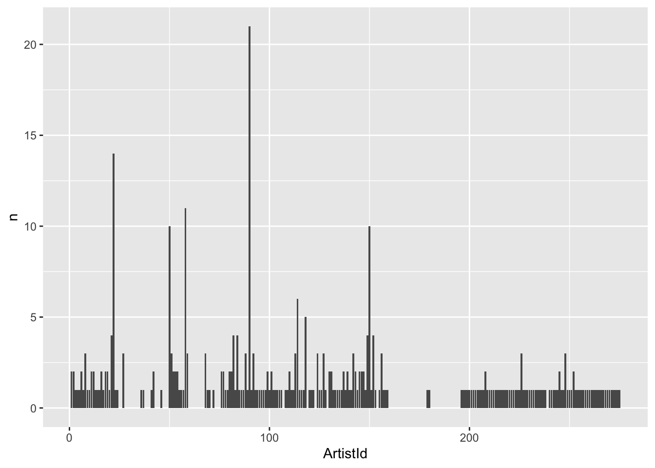

Let’s also extract the first letter from each album and plot the frequency of each letter.

tbl(connection, "Album") %>%
  mutate(first_letter = str_sub(Title, end = 1)) %>% 
  ggplot(aes(first_letter)) + 
  geom_bar()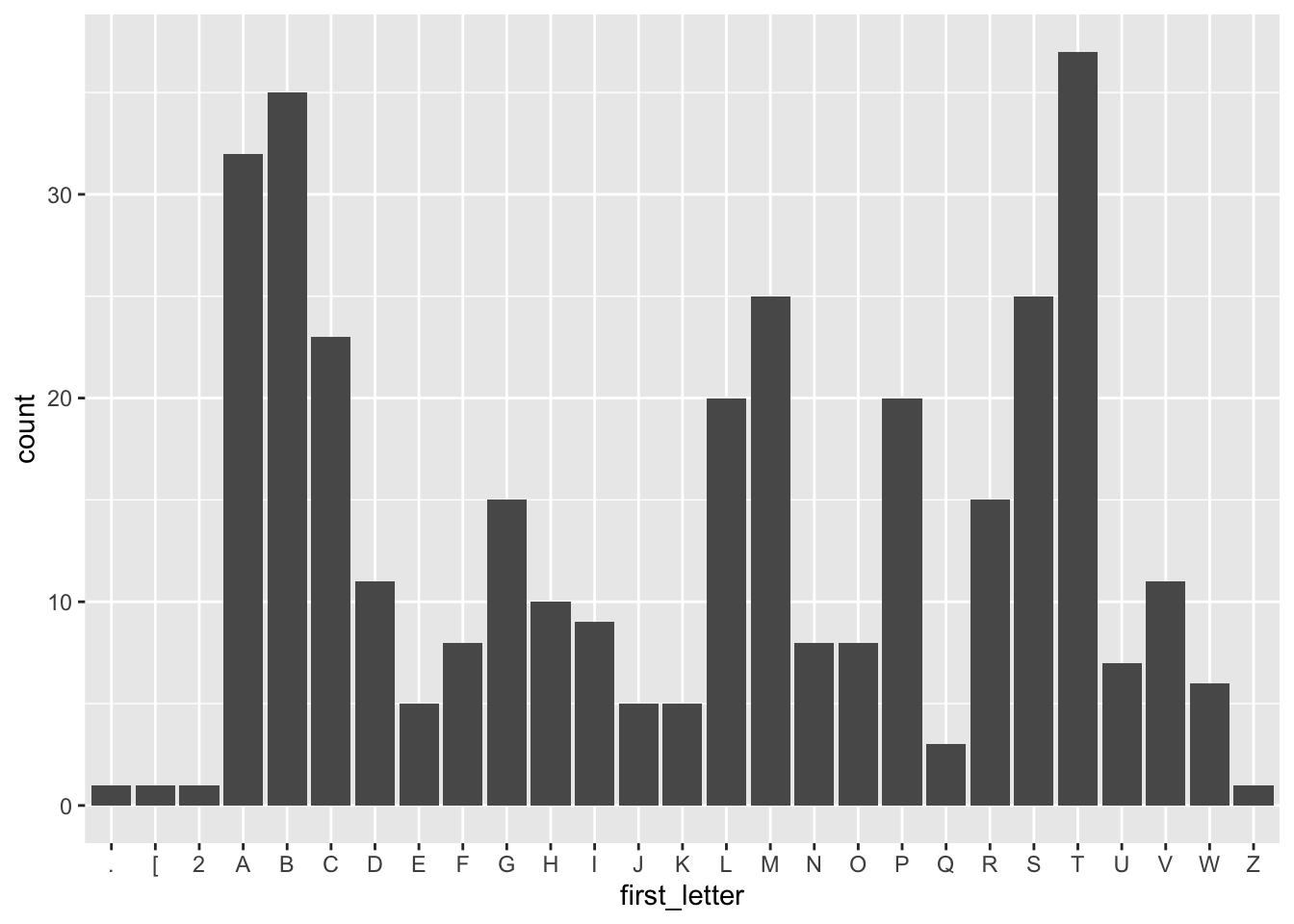

If you decide to make an album, you should try picking a less frequently used letter like E, J, K, Q, U, W, or Z!

Post-lecture materials

Final Questions

Here are some post-lecture questions to help you think about the material discussed.

Questions

Using the survey.db database:

Use .schema to identify column that contains integers
Write a query that selects only the name column from the Site table.
Many people format queries in the following two ways. What style do you find easiest to read, and why?

SELECT personal, family FROM person;

select Personal, Family from PERSON;

Write a query that selects distinct dates from the Visited table.
Write a query that displays the full names of the scientists in the Person table, ordered by family name.

Additional Resources

Tip

Pre-lecture materials

Read ahead

Acknowledgements

Learning objectives

Installation

Command-line tool sqlite3

R packages

Relational databases

Languages

SQL basics

Example data

SQL .tables and .schema

SQL command SELECT

More about SELECT

The * operator

Sorting and removing duplicates

Other important tasks

Filtering

And more

SQL in R

Connect to the SQL database

Example workflow

Database helper functions in R

SQL queries with dplyr

Example: album covers

Connect to the SQLite database

Using dplyr

data viz

Post-lecture materials

Final Questions

Additional Resources

Command-line tool `sqlite3`

SQL `.tables` and `.schema`

SQL command `SELECT`

More about `SELECT`

The `*` operator

SQL queries with `dplyr`

Using `dplyr`