Machine learning paradigms and workflows – Part 02

Overview of ML paradigms and workflows in R

Author

Affiliation

Stephanie Hicks

Department of Biostatistics, Johns Hopkins

Published

November 18, 2025

Pre-lecture activities

Tip

We will continue with tidymodels, so there is nothing else to install for the lecture. However, if you want to see a different linear regression model workflow with the penguins dataset, checkout this tutorial:

Regression in tidymodels

Lecture

Acknowledgements

Material for this lecture was borrowed and adopted from

An Introduction to Statistical Learning

Learning objectives

At the end of this lesson you will:

Use tidymodels as collection of packages for modeling and machine learning using tidyverse principles
Be able to fit a linear regression model and a random forest model to be used for prediction in supervised learning
Be able to split data into “train” and “test” to reduce overfitting and improve model performance

Slides

Lecture 07: Machine learning paradgims – Part 02

Class activity

For the rest of the time in class, we will practice implementing more ML models with the same penguins dataset.

Objectives of the activity

Extend the linear regression example using additional predictors and compare performance
Understand how a playing with hyperparameters can change model performance
Explore whether adding interaction terms improves predictions

For this in-class activity, you can work alone or find a partner. I encourage you to find a partner so you can discuss the questions asked below.

Part 1

Using penguins dataset discussed in class, we will first extend the linear regression example using additional predictors and compare the model performances. Using this dataset, build two linear regression models predicting body_mass_g using:

Model A: bill_length_mm + species
Model B: bill_length_mm + flipper_length_mm + species + sex

Use the same train/test split for both models. Then, compare RMSE and R^2 between Model A and Model B on:

the training set
the test set

Think about and discuss these questions with a partner (or to yourself):

Which model performs better?
Did adding predictors help?
Is there evidence of overfitting?

Solution

First, we will load libraries and split the data into train and test

# shared setup
library(tidymodels)
library(palmerpenguins)
library(dplyr)
library(ggplot2)
library(vip)

# feature engineering
penguins <- na.omit(penguins)

# create a single train/test split used for all problems
set.seed(123)
p_split <- initial_split(penguins, prop = 0.8)
p_train <- training(p_split)
p_test  <- testing(p_split)

# metrics set we will use later on
reg_metrics <- metric_set(rmse, rsq, mae)

Next, we will compare Model A vs Model B

# Model A: bill_length_mm + species
model_a <- linear_reg() %>% set_engine("lm") %>% set_mode("regression") %>%
  fit(body_mass_g ~ bill_length_mm + species, data = p_train)

# Model B: bill_length_mm + flipper_length_mm + species + sex
model_b <- linear_reg() %>% set_engine("lm") %>% set_mode("regression") %>%
  fit(body_mass_g ~ bill_length_mm + flipper_length_mm + species + sex, data = p_train)

# predictions and metrics on training set
pred_a_train <- predict(model_a, p_train) %>% bind_cols(p_train)
pred_b_train <- predict(model_b, p_train) %>% bind_cols(p_train)

metrics_a_train <- pred_a_train %>% reg_metrics(truth = body_mass_g, estimate = .pred)
metrics_b_train <- pred_b_train %>% reg_metrics(truth = body_mass_g, estimate = .pred)

# predictions and metrics on test set
pred_a_test <- predict(model_a, p_test) %>% bind_cols(p_test)
pred_b_test <- predict(model_b, p_test) %>% bind_cols(p_test)

metrics_a_test <- pred_a_test %>% reg_metrics(truth = body_mass_g, estimate = .pred)
metrics_b_test <- pred_b_test %>% reg_metrics(truth = body_mass_g, estimate = .pred)

# print results
cat("=== Model A: Training metrics ===\n"); print(metrics_a_train)

=== Model A: Training metrics ===

# A tibble: 3 × 3
  .metric .estimator .estimate
  <chr>   <chr>          <dbl>
1 rmse    standard     371.   
2 rsq     standard       0.790
3 mae     standard     292.

cat("\n=== Model B: Training metrics ===\n"); print(metrics_b_train)


=== Model B: Training metrics ===

# A tibble: 3 × 3
  .metric .estimator .estimate
  <chr>   <chr>          <dbl>
1 rmse    standard     287.   
2 rsq     standard       0.874
3 mae     standard     228.

cat("\n=== Model A: Test metrics ===\n"); print(metrics_a_test)


=== Model A: Test metrics ===

# A tibble: 3 × 3
  .metric .estimator .estimate
  <chr>   <chr>          <dbl>
1 rmse    standard     383.   
2 rsq     standard       0.764
3 mae     standard     317.

cat("\n=== Model B: Test metrics ===\n"); print(metrics_b_test)


=== Model B: Test metrics ===

# A tibble: 3 × 3
  .metric .estimator .estimate
  <chr>   <chr>          <dbl>
1 rmse    standard     300.   
2 rsq     standard       0.854
3 mae     standard     254.

# compare observed vs predicted on test set for Model B (more features)
ggplot(pred_b_test, aes(x = body_mass_g, y = .pred, color = species)) +
  geom_point(alpha = 0.8) +
  geom_abline(linetype = "dashed") +
  labs(title = "Model B: Observed vs Predicted on Test Set",
       x = "Observed body_mass_g", y = "Predicted .pred")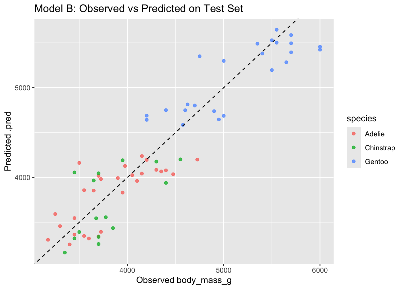

Generally:

if Model B improves test rmse (and not only train rmse), added predictors help generalization
if Model B reduces train rmse a lot, but test rmse does not improve (or worsens), that suggests overfitting

Part 2

In this question, we will use the training set from above, but now we will switch to random forests. There is an argument called mtry = 3 used to identify the number of features sampled for each tree. Let’s try changing it and we can “tune” the this parameter (also known as a “hyperparameter”). We will ask if this changes the model’s performance.

Using the training dataset, fit three random forest models with different mtry values:

mtry = 2
mtry = 3
mtry = 5

For each model:

Fit on the training data
Evaluate on the test data (e.g. rmse and rsq)
Plot mtry vs test rmse.

Think about and discuss these questions with a partner (or to yourself):

Which mtry yields the lowest test rmse?
Why might increasing mtry help or hurt performance?

Solution

library(purrr)
library(tidyr)

# model set up
rf_formula <- body_mass_g ~ bill_length_mm + flipper_length_mm + sex + species

# set up a vector of mtry values (will use purrr for this)
mtry_values <- c(2, 3, 5)

# function to fit random forest and return test metrics
fit_rf_and_eval <- function(mtry_val) {
  spec <- rand_forest(mtry = mtry_val, trees = 500) %>%
    set_engine("ranger", importance = "impurity") %>%
    set_mode("regression")
  
  fit_obj <- spec %>% fit(rf_formula, data = p_train)
  
  pred_test <- predict(fit_obj, p_test) %>% bind_cols(p_test)
  met_test <- pred_test %>% reg_metrics(truth = body_mass_g, estimate = .pred) %>%
    filter(.metric %in% c("rmse", "rsq", "mae")) %>%
    mutate(mtry = mtry_val, set = "test")
  
  # also return training metrics optionally
  pred_train <- predict(fit_obj, p_train) %>% bind_cols(p_train)
  met_train <- pred_train %>% reg_metrics(truth = body_mass_g, estimate = .pred) %>%
    filter(.metric %in% c("rmse", "rsq", "mae")) %>%
    mutate(mtry = mtry_val, set = "train")
  
  bind_rows(met_train, met_test)
}

results_list <- map(mtry_values, fit_rf_and_eval)

Warning: ! 5 columns were requested but there were 4 predictors in the data.
ℹ 4 predictors will be used.

results_df <- bind_rows(results_list)

# make it into a nice table to compare all the metrics
print(results_df %>% pivot_wider(names_from = c(set, .metric), values_from = .estimate))

# A tibble: 3 × 8
  .estimator  mtry train_rmse train_rsq train_mae test_rmse test_rsq test_mae
  <chr>      <dbl>      <dbl>     <dbl>     <dbl>     <dbl>    <dbl>    <dbl>
1 standard       2       193.     0.944      153.      316.    0.840     257.
2 standard       3       157.     0.963      124.      334.    0.825     269.
3 standard       5       150.     0.966      119.      335.    0.825     269.

Finally, we plot mtry vs test rmse

results_df %>%
  filter(set == "test", .metric == "rmse") %>%
  ggplot(aes(x = factor(mtry), y = .estimate, group = 1)) +
  geom_point(size = 3) + geom_line() +
  labs(title = "test rmse vs mtry (random forest)",
       x = "mtry", y = "test rmse")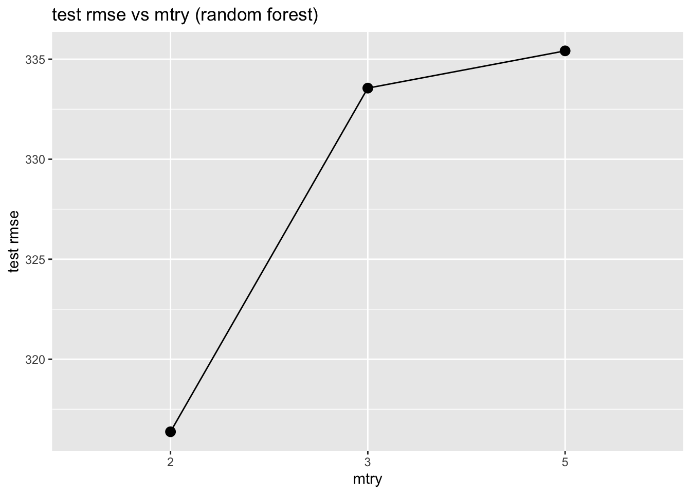

Generally:

Small mtry reduces correlation between trees and may reduce overfitting
Large mtry lets trees be more similar to full trees (may reduce bias but increase variance)

Part 3

In this question, fit two linear regression models to predict body_mass_g:

Model without interaction: body_mass_g ~ bill_length_mm + flipper_length_mm + species
Model with interaction: body_mass_g ~ bill_length_mm * species + flipper_length_mm

You want want to compare both models on the train and test rmse. Then, create a visualization of predicted vs actual body mass for the test set for each model.

Think about and discuss these questions with a partner (or to yourself):

Did adding interactions help?
Why might interactions between bill_length_mm and species matter biologically?

Solution

# model without interaction
model_no_int <- linear_reg() %>% set_engine("lm") %>% fit(
  body_mass_g ~ bill_length_mm + flipper_length_mm + species,
  data = p_train
)

# model with interaction between bill_length_mm and species
model_int <- linear_reg() %>% set_engine("lm") %>% fit(
  body_mass_g ~ bill_length_mm * species + flipper_length_mm,
  data = p_train
)

# evaluate on train set
pred_no_int_train <- predict(model_no_int, p_train) %>% bind_cols(p_train)
pred_int_train    <- predict(model_int, p_train) %>% bind_cols(p_train)

metrics_no_int_train <- pred_no_int_train %>% reg_metrics(truth = body_mass_g, estimate = .pred)
metrics_int_train    <- pred_int_train %>% reg_metrics(truth = body_mass_g, estimate = .pred)

# evaluate on test set
pred_no_int_test <- predict(model_no_int, p_test) %>% bind_cols(p_test)
pred_int_test    <- predict(model_int, p_test) %>% bind_cols(p_test)

metrics_no_int_test <- pred_no_int_test %>% reg_metrics(truth = body_mass_g, estimate = .pred)
metrics_int_test    <- pred_int_test %>% reg_metrics(truth = body_mass_g, estimate = .pred)

# print results
cat("=== No interaction: Training ===\n"); print(metrics_no_int_train)

=== No interaction: Training ===

# A tibble: 3 × 3
  .metric .estimator .estimate
  <chr>   <chr>          <dbl>
1 rmse    standard     336.   
2 rsq     standard       0.828
3 mae     standard     266.

cat("\n=== Interaction: Training ===\n"); print(metrics_int_train)


=== Interaction: Training ===

# A tibble: 3 × 3
  .metric .estimator .estimate
  <chr>   <chr>          <dbl>
1 rmse    standard     331.   
2 rsq     standard       0.832
3 mae     standard     259.

cat("\n=== No interaction: Test ===\n"); print(metrics_no_int_test)


=== No interaction: Test ===

# A tibble: 3 × 3
  .metric .estimator .estimate
  <chr>   <chr>          <dbl>
1 rmse    standard     342.   
2 rsq     standard       0.811
3 mae     standard     279.

cat("\n=== Interaction: Test ===\n"); print(metrics_int_test)


=== Interaction: Test ===

# A tibble: 3 × 3
  .metric .estimator .estimate
  <chr>   <chr>          <dbl>
1 rmse    standard     345.   
2 rsq     standard       0.807
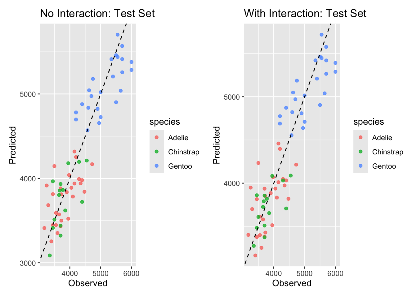
3 mae     standard     282.

Finally, let’s visualize

# visualization: test set predicted vs observed for both models
p1 <- ggplot(pred_no_int_test, aes(x = body_mass_g, y = .pred, color = species)) +
  geom_point(alpha = 0.8) + geom_abline(lty = 2) +
  labs(title = "No Interaction: Test Set", x = "Observed", y = "Predicted")

p2 <- ggplot(pred_int_test, aes(x = body_mass_g, y = .pred, color = species)) +
  geom_point(alpha = 0.8) + geom_abline(lty = 2) +
  labs(title = "With Interaction: Test Set", x = "Observed", y = "Predicted")

# Print side-by-side (requires patchwork or cowplot). If not available, print separately.
if (requireNamespace("patchwork", quietly = TRUE)) {
  print(p1 + p2)
} else {
  print(p1); print(p2)
}

# Optional: inspect interaction coefficients
tidy(model_int)

# A tibble: 7 × 5
  term                            estimate std.error statistic  p.value
  <chr>                              <dbl>     <dbl>     <dbl>    <dbl>
1 (Intercept)                      -4473.     725.      -6.17  2.57e- 9
2 bill_length_mm                      83.3     12.6      6.60  2.37e-10
3 speciesChinstrap                  1465.     825.       1.78  7.69e- 2
4 speciesGentoo                      717.     706.       1.01  3.11e- 1
5 flipper_length_mm                   26.0      3.45     7.52  9.01e-13
6 bill_length_mm:speciesChinstrap    -49.8     18.5     -2.69  7.56e- 3
7 bill_length_mm:speciesGentoo       -16.1     16.6     -0.972 3.32e- 1

Generally:

if the interaction model lowers test RMSE, the interaction helped generalization. here, the interaction term allows the slope between bill length and body mass to differ by species — biologically reasonable if species have different scaling relationships.
also it’s worth checking whether the interaction model greatly improves training fit but not test fit (overfitting warning).