3 Construction of expression matrix

Many analyses of scRNA-seq data take as their starting point an expression matrix. By convention, the each row of the expression matrix represents a gene and each column represents a cell (although some authors use the transpose). Each entry represents the expression level of a particular gene in a given cell. The units by which the expression is meassured depends on the protocol and the normalization strategy used.

In this section, we will describe how to go from a set of raw sequencing reads to an expression matrix.

3.1 Raw sequencing reads QC

3.1.1 FastQ

The output from a scRNA-seq experiment is a large collection of cDNA reads. FastQ is the most raw form of scRNA-seq data you will encounter. The first step is to ensure that the reads are of high quality.

All scRNA-seq protocols are sequenced with paired-end sequencing. Barcode sequences may occur in one or both reads depending on the protocol employed. However, protocols using unique molecular identifiers (UMIs) will generally contain one read with the cell and UMI barcodes plus adapters but without any transcript sequence. Thus reads will be mapped as if they are single-end sequenced despite actually being paired end.

3.1.2 Check the quality of the raw sequencing reads

FastQC is a good tool for this. This software produces a FastQC report than be used to evaluate questions such as How good quality are the reads? Is there anything we should be concerned about?, etc.

3.1.3 Trim sequencing adapaters from sequencing reads

For example, Trim Galore! is wrapper for trimming reads from FastQ files using cutadapt. Once you trim the adapaters, you can re-run FastQC to confirm successful removal.

3.2 Reads alignment

After trimming low quality bases from the reads, the remaining sequences can be mapped to a reference genome. Again, there is no need for a special purpose method for this, so we can use the STAR or the TopHat aligner. For large full-transcript datasets from well annotated organisms (e.g. mouse, human) pseudo-alignment methods (e.g. Kallisto, Salmon) may out-perform conventional alignment. For drop-seq based datasets with tens- or hundreds of thousands of reads pseudoaligners become more appealing since their run-time can be several orders of magnitude less than traditional aligners.

3.2.1 Genome (`FASTA`, `GTF`)

To map your reads you will need the reference genome and in many cases the genome annotation file (in either GTF or GFF format). These can be downloaded for model organisms from any of the main genomics databases: Ensembl, NCBI, or UCSC Genome Browser.

GTF files contain annotations of genes, transcripts, and exons. They must contain:

seqname : chromosome/scaffold
source : where this annotation came from
feature : what kind of feature is this? (e.g. gene, transcript, exon)
start : start position (bp)
end : end position (bp)
score : a number
strand : + (forward) or - (reverse)
frame : if CDS indicates which base is the first base of the first codon (0 = first base, 1 = second base, etc..)
attribute : semicolon-separated list of tag-value pairs of extra information (e.g. names/IDs, biotype)

Empty fields are marked with “.”

In our experience:

Ensembl is the easiest of these to use, and has the largest set of annotations
NCBI tends to be more strict in including only high confidence gene annotations
Whereas UCSC contains multiple geneset annotations that use different criteria

If your experimental system includes non-standard sequences these must be added to both the genome fasta and gtf to quantify their expression. Most commonly this is done for the ERCC spike-ins, although the same must be done for CRISPR- related sequences or other overexpression/reporter constructs.

3.2.2 Alignment using Star

An example of how to map reads.fq (the .gz means the file is zipped) using STAR is

$<path_to_STAR>/STAR --runThreadN 1 --runMode alignReads
--readFilesIn reads1.fq.gz reads2.fq.gz --readFilesCommand zcat --genomeDir <path>
--parametersFiles FileOfMoreParameters.txt --outFileNamePrefix <outpath>/output

Note, if the spike-ins are used, the reference sequence should be augmented with the DNA sequence of the spike-in molecules prior to mapping.

Note, when UMIs are used, their barcodes should be removed from the read sequence. A common practice is to add the barcode to the read name.

Once the reads for each cell have been mapped to the reference genome, we need to make sure that a sufficient number of reads from each cell could be mapped to the reference genome. In our experience, the fraction of mappable reads for mouse or human cells is 60-70%. However, this result may vary depending on protocol, read length and settings for the read alignment. As a general rule, we expect all cells to have a similar fraction of mapped reads, so any outliers should be inspected and possibly removed. A low proportion of mappable reads usually indicates contamination.

3.2.3 Pseudo-alignment using Salmon

An example of how to quantify expression using Salmon is

$<path_to_Salmon>/salmon quant -i salmon_transcript_index -1 
    reads1.fq.gz -2 reads2.fq.gz -p #threads -l A -g genome.gtf 
    --seqBias --gcBias --posBias

Note Salmon produces estimated read counts and estimated transcripts per million (tpm) in our experience the latter over corrects the expression of long genes for scRNA-seq, thus we recommend using read counts.

3.2.4 Mapped reads: `BAM` file format

BAM file format stores mapped reads in a standard and efficient manner. The human-readable version is called a SAM file, while the BAM file is the highly compressed version. BAM/SAM files contain a header which typically includes
information on the sample preparation, sequencing and mapping; and a tab-separated row for each individual alignment of each read.

BAM/SAM files can be converted to the other format using ‘samtools’:

3.2.4.1 Checking read quality from `BAM` file

Assuming that our reads are in experiment.bam, we can run FastQC as

<path_to_fastQC>/fastQC experiment.bam

Below is an example of the output from FastQC for a dataset of 125 bp reads. The plot reveals a technical error which resulted in a couple of bases failing to be read correctly in the centre of the read. However, since the rest of the read was of high quality this error will most likely have a negligible effect on mapping efficiency.

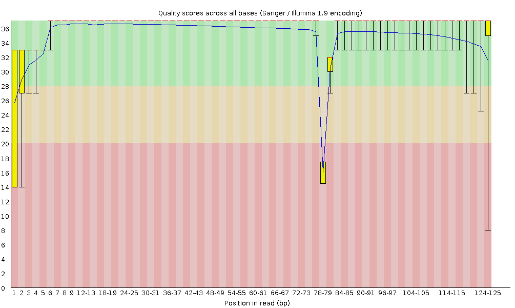
Figure 3.1: Example of FastQC output

Additionally, it is often helpful to visualize the data using the Integrative Genomics Browser (IGV) or SeqMonk tools.

3.2.5 CRAM

CRAM files are similar to BAM files only they contain information in the header to the reference genome used in the mapping in the header. This allow the bases in each read that are identical to the reference to be further compressed. CRAM also supports some data compression approaches to further optimize storage compared to BAMs. CRAMs are mainly used by the Sanger/EBI sequencing facility.

3.2.6 Reads Mapping QC

3.2.6.1 Total number of reads mapped to each cell

The histogram below shows the total number of reads mapped to each cell for an scRNA-seq experiment. Each bar represents one cell, and they have been sorted in ascending order by the total number of reads per cell. The three red arrows indicate cells that are outliers in terms of their coverage and they should be removed from further analysis. The two yellow arrows point to cells with a surprisingly large number of unmapped reads. In this example we kept the cells during the alignment QC step, but they were later removed during cell QC due to a high proportion of ribosomal RNA reads.

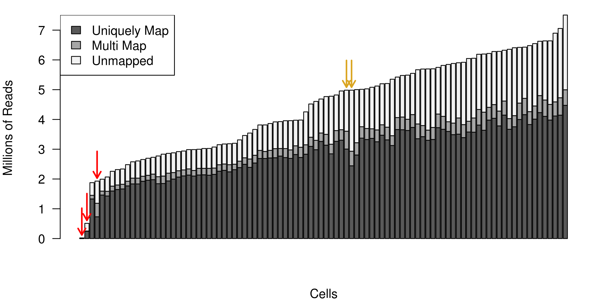
Figure 3.2: Example of the total number of reads mapped to each cell.

3.2.6.2 Mapping quality

After mapping the raw sequencing to the genome we need to evaluate the quality of the mapping. There are many ways to measure the mapping quality, including: amount of reads mapping to rRNA/tRNAs, proportion of uniquely mapping reads, reads mapping across splice junctions, read depth along the transcripts. Methods developed for bulk RNA-seq, such as RSeQC, are applicable to single-cell data.

However the expected results will depend on the experimental protocol, e.g. many scRNA-seq methods use poly-A selection to avoid sequencing rRNAs which results in a 3’ bias in the read coverage across the genes (aka gene body coverage). The figure below shows this 3’ bias as well as three cells which were outliers and removed from the dataset:

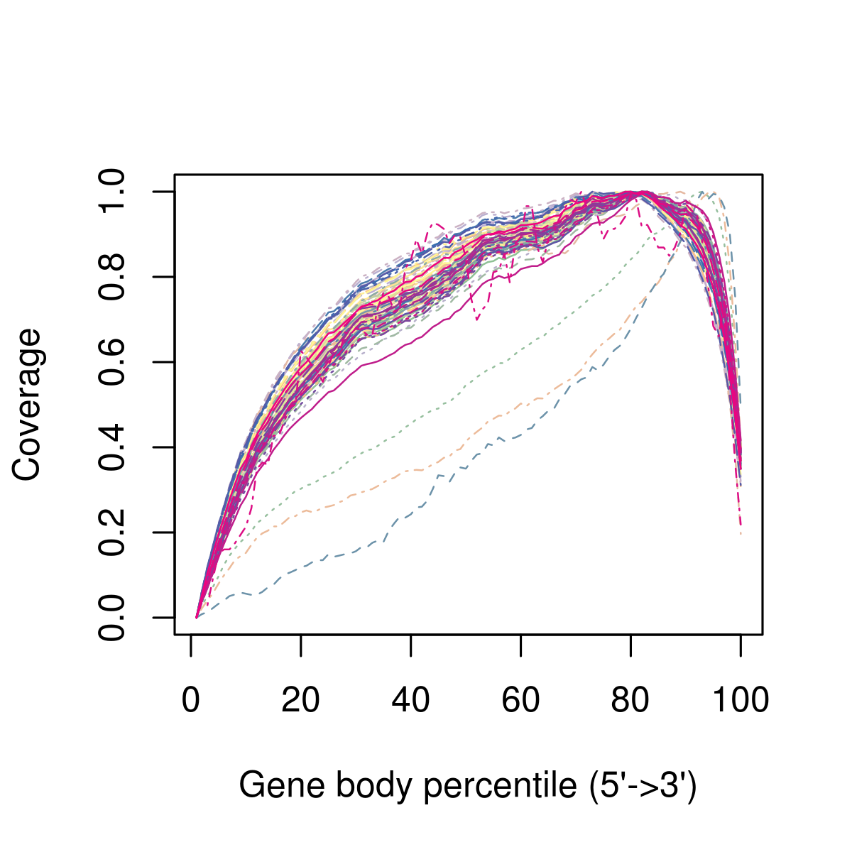
Figure 3.3: Example of the 3’ bias in the read coverage.

3.3 Reads quantification

The next step is to quantify the expression level of each gene for each cell. For mRNA data, we can use one of the tools which has been developed for bulk RNA-seq data, e.g. HT-seq or FeatureCounts (can read about parameters in user guide here).

# include multimapping
<featureCounts_path>/featureCounts -O -M -Q 30 -p -a genome.gtf -o outputfile input.bam
# exclude multimapping
<featureCounts_path>/featureCounts -Q 30 -p -a genome.gtf -o outputfile input.bam

Unique molecular identifiers (UMIs) make it possible to count the absolute number of molecules and they have proven popular for scRNA-seq.

3.4 Unique Molecular Identifiers (UMIs)

Unique Molecular Identifiers are short (4-10bp) random barcodes added to transcripts during reverse-transcription. They enable sequencing reads to be assigned to individual transcript molecules and thus the removal of amplification noise and biases from scRNASeq data.

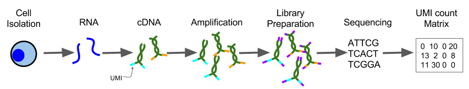
Figure 3.4: UMI sequencing protocol

When sequencing UMI containing data, techniques are used to specifically sequence only the end of the transcript containing the UMI (usually the 3’ end).

For more information processing reads from a UMI experiment, including mapping and counting barcodes, I refer you to the UMI chapter in original course material.

However, determining how to best process and use UMIs is currently an active area of research in the bioinformatics community. We are aware of several methods that have recently been developed, including: