Introduction to Single-Cell
Stephanie Hicks
intro-single-cell-01.RmdOverview
Key resources
- Workshop material: pkgdown website
- Code: GitHub
Part 1
Learning objectives
- Understand how count matrices are created from single-cell experimental platforms and protocols
- Recognize which basic principles and concepts were transfered from bulk to single-cell data analyses
- Understand the key differences between bulk and single-cell data
- Define what is a “Unique Molecular Identifier”
- Define multiplexing (and demultiplexing)
Part 2
Learning objectives
- Be able to create a count matrix and read it into R
- Recognize and define the
SingleCellExperimentS4 class in R/Bioconductor to store single-cell data - Understand strategies to get access to existing single-cell data in R
Overview
NGS data from scRNA-seq experiments must be converted into a matrix of expression values. This is usually a count matrix containing the number of reads (or UMIs) mapped to each gene (row) in each cell (column). Once this quantification is complete, we can proceed with our downstream statistical analyses in R.
Constructing a count matrix from raw scRNA-seq data requires some thought as the term “single-cell RNA-seq” encompasses a variety of different experimental protocols. This includes
- droplet-based protocols like 10X Genomics, inDrop and Drop-seq
- plate-based protocols with UMIs like CEL-seq(2) and MARS-seq
- plate-based protocols with reads (mostly Smart-seq2)
- others like sciRNA-seq, etc
Each approach requires a different processing pipeline to deal with cell demultiplexing and UMI deduplication (if applicable). Here, we will briefly describe some of the methods used to generate a count matrix and read it into R.
Creating a count matrix
As mentioned above, the exact procedure for quantifying expression depends on the technology involved:
- For 10X Genomics data, the
Cellrangersoftware suite (Zheng et al. 2017) provides a custom pipeline to obtain a count matrix. This uses STAR to align reads to the reference genome and then counts the number of unique UMIs mapped to each gene. - Alternatively, pseudo-alignment methods such as
alevin(Srivastava et al. 2019) can be used to obtain a count matrix from the same data. This avoids the need for explicit alignment, which reduces the compute time and memory usage. - For other highly multiplexed protocols, the
scPipepackage provides a more general pipeline for processing scRNA-seq data. This uses the Rsubread aligner to align reads and then counts reads or UMIs per gene. - For CEL-seq or CEL-seq2 data, the
scruffpackage provides a dedicated pipeline for quantification. - For read-based protocols, we can generally re-use the same pipelines for processing bulk RNA-seq data (e.g. Subread, RSEM, salmon)
- For any data involving spike-in transcripts, the spike-in sequences should be included as part of the reference genome during alignment and quantification.
In all cases, the identity of the genes in the count matrix should be defined with standard identifiers from Ensembl or Entrez. These provide an unambiguous mapping between each row of the matrix and the corresponding gene.
In contrast, a single gene symbol may be used by multiple loci, or the mapping between symbols and genes may change over time, e.g., if the gene is renamed. This makes it difficult to re-use the count matrix as we cannot be confident in the meaning of the symbols. (Of course, identifiers can be easily converted to gene symbols later on in the analysis. This is the recommended approach as it allows us to document how the conversion was performed and to backtrack to the stable identifiers if the symbols are ambiguous.)
SingleCellExperiment Class
One of the main strengths of the Bioconductor project lies in the use
of a common data infrastructure that powers interoperability across
packages. Users should be able to analyze their data using functions
from different Bioconductor packages without the need to convert between
formats. To this end, the SingleCellExperiment class (from
the SingleCellExperiment package) serves as the common
currency for data exchange across 70+ single-cell-related Bioconductor
packages. This class implements a data structure that stores all aspects
of our single-cell data - gene-by-cell expression data, per-cell
metadata and per-gene annotation - and manipulate them in a synchronized
manner.
Amezquita et al. 2019 (https://doi.org/10.1101/590562)
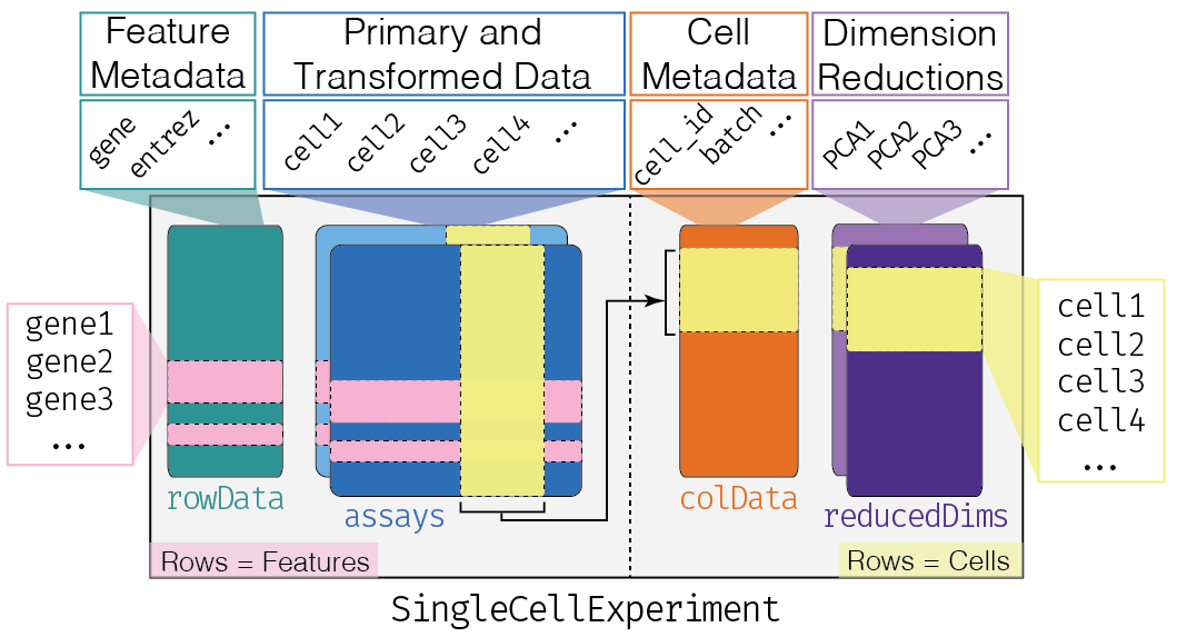
Each piece of (meta)data in the SingleCellExperiment is
represented by a separate “slot”. (This terminology comes from the S4
class system, but that’s not important right now.) If we imagine the
SingleCellExperiment object to be a cargo ship, the slots
can be thought of as individual cargo boxes with different contents,
e.g., certain slots expect numeric matrices whereas others may expect
data frames.
If you want to know more about the available slots, their expected formats, and how we can interact with them, check out this chapter.
SingleCellExperiment Example
Let’s show you what a SingleCellExperiment (or
sce for short) looks like.
sce## class: SingleCellExperiment
## dim: 20006 3005
## metadata(0):
## assays(1): counts
## rownames(20006): Tspan12 Tshz1 ... mt-Rnr1 mt-Nd4l
## rowData names(1): featureType
## colnames(3005): 1772071015_C02 1772071017_G12 ... 1772066098_A12
## 1772058148_F03
## colData names(10): tissue group # ... level1class level2class
## reducedDimNames(0):
## mainExpName: endogenous
## altExpNames(2): ERCC repeatThis SingleCellExperiment object has 20006 genes and
3005 cells.
We can pull out the counts matrix with the counts()
function and the corresponding rowData() and
colData():
counts(sce)[1:5, 1:5]## 1772071015_C02 1772071017_G12 1772071017_A05 1772071014_B06
## Tspan12 0 0 0 3
## Tshz1 3 1 0 2
## Fnbp1l 3 1 6 4
## Adamts15 0 0 0 0
## Cldn12 1 1 1 0
## 1772067065_H06
## Tspan12 0
## Tshz1 2
## Fnbp1l 1
## Adamts15 0
## Cldn12 0
rowData(sce)## DataFrame with 20006 rows and 1 column
## featureType
## <character>
## Tspan12 endogenous
## Tshz1 endogenous
## Fnbp1l endogenous
## Adamts15 endogenous
## Cldn12 endogenous
## ... ...
## mt-Co2 mito
## mt-Co1 mito
## mt-Rnr2 mito
## mt-Rnr1 mito
## mt-Nd4l mito
colData(sce)## DataFrame with 3005 rows and 10 columns
## tissue group # total mRNA mol well sex
## <character> <numeric> <numeric> <numeric> <numeric>
## 1772071015_C02 sscortex 1 1221 3 3
## 1772071017_G12 sscortex 1 1231 95 1
## 1772071017_A05 sscortex 1 1652 27 1
## 1772071014_B06 sscortex 1 1696 37 3
## 1772067065_H06 sscortex 1 1219 43 3
## ... ... ... ... ... ...
## 1772067059_B04 ca1hippocampus 9 1997 19 1
## 1772066097_D04 ca1hippocampus 9 1415 21 1
## 1772063068_D01 sscortex 9 1876 34 3
## 1772066098_A12 ca1hippocampus 9 1546 88 1
## 1772058148_F03 sscortex 9 1970 15 3
## age diameter cell_id level1class level2class
## <numeric> <numeric> <character> <character> <character>
## 1772071015_C02 2 1 1772071015_C02 interneurons Int10
## 1772071017_G12 1 353 1772071017_G12 interneurons Int10
## 1772071017_A05 1 13 1772071017_A05 interneurons Int6
## 1772071014_B06 2 19 1772071014_B06 interneurons Int10
## 1772067065_H06 6 12 1772067065_H06 interneurons Int9
## ... ... ... ... ... ...
## 1772067059_B04 4 382 1772067059_B04 endothelial-mural Peric
## 1772066097_D04 7 12 1772066097_D04 endothelial-mural Vsmc
## 1772063068_D01 7 268 1772063068_D01 endothelial-mural Vsmc
## 1772066098_A12 7 324 1772066098_A12 endothelial-mural Vsmc
## 1772058148_F03 7 6 1772058148_F03 endothelial-mural VsmcData resources
In this section, we will discuss data packages and website for where to get existing single-cell data
HCAData data package
The HCAData package allows a direct access to the
dataset generated by the Human Cell Atlas project for further processing
in R and Bioconductor. It does so by providing the datasets as
SingleCellExperiment objects. The datasets use
HDF5Array package to avoid loading the entire data set in
memory. Instead, it stores the counts on disk as a .HDF5
file, and loads subsets of the data into memory upon request.
The datasets are otherwise available in other formats (also as raw data) at this link: http://preview.data.humancellatlas.org/.
The HCAData() function downloads the relevant files from
ExperimentHub. If no argument is provided, a list of the
available datasets is returned, specifying which name to enter as
dataset parameter when calling HCAData.
If we specify either ica_bone_marrow or
ica_cord_blood in the function, we get returend a
SingleCellExperiment object
sce_bonemarrow <- HCAData("ica_bone_marrow")
sce_bonemarrow
## class: SingleCellExperiment
## dim: 33694 378000
## metadata(0):
## assays(1): counts
## rownames(33694): ENSG00000243485 ENSG00000237613 ... ENSG00000277475
## ENSG00000268674
## rowData names(2): ID Symbol
## colnames(378000): MantonBM1_HiSeq_1-AAACCTGAGCAGGTCA-1
## MantonBM1_HiSeq_1-AAACCTGCACACTGCG-1 ...
## MantonBM8_HiSeq_8-TTTGTCATCTGCCAGG-1
## MantonBM8_HiSeq_8-TTTGTCATCTTGAGAC-1
## colData names(1): Barcode
## reducedDimNames(0):
## mainExpName: NULL
## altExpNames(0):We can see even though it’s a lot cells, this is actually quite small
of an object in terms of data read into memory. This is due to the magic
of HDF5Array and DelayedArray.
pryr::object_size(sce_bonemarrow)## 44.17 MB
hca data package
The HCAData package only has two datasets from the Human
Cell Atlas, but for a comprehensive list fromt he HCA Data Coordinating
Platform, check out the hca R/Bioconductor package (http://www.bioconductor.org/packages/hca).
scRNAseq data package
The scRNAseq package provides convenient access to
several publicly available data sets in the form of
SingleCellExperiment objects. The focus of this package is
to capture datasets that are not easily read into R with a one-liner
from, e.g., read.csv(). Instead, we do the necessary data munging so
that users only need to call a single function to obtain a well-formed
SingleCellExperiment.
library(scRNAseq)
sce <- ZeiselBrainData()
sce
## class: SingleCellExperiment
## dim: 20006 3005
## metadata(0):
## assays(1): counts
## rownames(20006): Tspan12 Tshz1 ... mt-Rnr1 mt-Nd4l
## rowData names(1): featureType
## colnames(3005): 1772071015_C02 1772071017_G12 ... 1772066098_A12
## 1772058148_F03
## colData names(10): tissue group # ... level1class level2class
## reducedDimNames(0):
## mainExpName: endogenous
## altExpNames(2): ERCC repeatTo see the list of available datasets, use the
listDatasets() function:
out <- listDatasets()
out
## DataFrame with 61 rows and 5 columns
## Reference Taxonomy Part Number
## <character> <integer> <character> <integer>
## 1 @aztekin2019identifi.. 8355 tail 13199
## 2 @bach2017differentia.. 10090 mammary gland 25806
## 3 @bacher2020low 9606 T cells 104417
## 4 @baron2016singlecell 9606 pancreas 8569
## 5 @baron2016singlecell 10090 pancreas 1886
## ... ... ... ... ...
## 57 @zeisel2018molecular 10090 nervous system 160796
## 58 @zhao2020singlecell 9606 liver immune cells 68100
## 59 @zhong2018singlecell 9606 prefrontal cortex 2394
## 60 @zilionis2019singlec.. 9606 lung 173954
## 61 @zilionis2019singlec.. 10090 lung 17549
## Call
## <character>
## 1 AztekinTailData()
## 2 BachMammaryData()
## 3 BacherTCellData()
## 4 BaronPancreasData('h..
## 5 BaronPancreasData('m..
## ... ...
## 57 ZeiselNervousData()
## 58 ZhaoImmuneLiverData()
## 59 ZhongPrefrontalData()
## 60 ZilionisLungData()
## 61 ZilionisLungData('mo..If the original dataset was not provided with Ensembl annotation, we
can map the identifiers with ensembl=TRUE. Any genes
without a corresponding Ensembl identifier is discarded
from the dataset.
sce <- ZeiselBrainData(ensembl=TRUE)
head(rownames(sce))
## [1] "ENSMUSG00000029669" "ENSMUSG00000046982" "ENSMUSG00000039735"
## [4] "ENSMUSG00000033453" "ENSMUSG00000046798" "ENSMUSG00000034009"Functions also have a location=TRUE argument that loads
in the gene coordinates.
sce <- ZeiselBrainData(ensembl=TRUE, location=TRUE)
head(rowRanges(sce))
## GRanges object with 6 ranges and 2 metadata columns:
## seqnames ranges strand | featureType
## <Rle> <IRanges> <Rle> | <character>
## ENSMUSG00000029669 6 21771395-21852515 - | endogenous
## ENSMUSG00000046982 18 84011627-84087706 - | endogenous
## ENSMUSG00000039735 3 122538719-122619715 - | endogenous
## ENSMUSG00000033453 9 30899155-30922452 - | endogenous
## ENSMUSG00000046798 5 5489537-5514958 - | endogenous
## ENSMUSG00000034009 3 79641611-79737880 - | endogenous
## originalName
## <character>
## ENSMUSG00000029669 Tspan12
## ENSMUSG00000046982 Tshz1
## ENSMUSG00000039735 Fnbp1l
## ENSMUSG00000033453 Adamts15
## ENSMUSG00000046798 Cldn12
## ENSMUSG00000034009 Rxfp1
## -------
## seqinfo: 118 sequences (1 circular) from GRCm38 genomeSession Info
## R version 4.2.1 (2022-06-23)
## Platform: aarch64-apple-darwin21.5.0 (64-bit)
## Running under: macOS Monterey 12.4
##
## Matrix products: default
## BLAS:   /opt/homebrew/Cellar/openblas/0.3.20/lib/libopenblasp-r0.3.20.dylib
## LAPACK: /opt/homebrew/Cellar/r/4.2.1/lib/R/lib/libRlapack.dylib
##
## locale:
## [1] en_US.UTF-8/en_US.UTF-8/en_US.UTF-8/C/en_US.UTF-8/en_US.UTF-8
##
## attached base packages:
## [1] stats4    stats     graphics  grDevices utils     datasets  methods
## [8] base
##
## other attached packages:
##  [1] ensembldb_2.20.2            AnnotationFilter_1.20.0
##  [3] GenomicFeatures_1.48.3      AnnotationDbi_1.58.0
##  [5] rhdf5_2.40.0                HCAData_1.12.0
##  [7] scRNAseq_2.10.0             scater_1.24.0
##  [9] ggplot2_3.3.6               scuttle_1.6.2
## [11] SingleCellExperiment_1.18.0 SummarizedExperiment_1.26.1
## [13] Biobase_2.56.0              GenomicRanges_1.48.0
## [15] GenomeInfoDb_1.32.2         IRanges_2.30.0
## [17] S4Vectors_0.34.0            BiocGenerics_0.42.0
## [19] MatrixGenerics_1.8.1        matrixStats_0.62.0
##
## loaded via a namespace (and not attached):
##   [1] AnnotationHub_3.4.0           BiocFileCache_2.4.0
##   [3] systemfonts_1.0.4             lazyeval_0.2.2
##   [5] BiocParallel_1.30.3           pryr_0.1.5
##   [7] digest_0.6.29                 htmltools_0.5.2
##   [9] viridis_0.6.2                 fansi_1.0.3
##  [11] magrittr_2.0.3                memoise_2.0.1
##  [13] ScaledMatrix_1.4.0            Biostrings_2.64.0
##  [15] pkgdown_2.0.5                 prettyunits_1.1.1
##  [17] colorspace_2.0-3              blob_1.2.3
##  [19] rappdirs_0.3.3                ggrepel_0.9.1
##  [21] lobstr_1.1.2                  textshaping_0.3.6
##  [23] xfun_0.31                     dplyr_1.0.9
##  [25] crayon_1.5.1                  RCurl_1.98-1.7
##  [27] jsonlite_1.8.0                glue_1.6.2
##  [29] gtable_0.3.0                  zlibbioc_1.42.0
##  [31] XVector_0.36.0                DelayedArray_0.22.0
##  [33] BiocSingular_1.12.0           Rhdf5lib_1.18.2
##  [35] HDF5Array_1.24.1              scales_1.2.0
##  [37] DBI_1.1.3                     Rcpp_1.0.8.3
##  [39] viridisLite_0.4.0             xtable_1.8-4
##  [41] progress_1.2.2                bit_4.0.4
##  [43] rsvd_1.0.5                    httr_1.4.3
##  [45] ellipsis_0.3.2                pkgconfig_2.0.3
##  [47] XML_3.99-0.10                 sass_0.4.1
##  [49] dbplyr_2.2.1                  utf8_1.2.2
##  [51] tidyselect_1.1.2              rlang_1.0.3
##  [53] later_1.3.0                   munsell_0.5.0
##  [55] BiocVersion_3.15.2            tools_4.2.1
##  [57] cachem_1.0.6                  cli_3.3.0
##  [59] generics_0.1.3                RSQLite_2.2.14
##  [61] ExperimentHub_2.4.0           evaluate_0.15
##  [63] stringr_1.4.0                 fastmap_1.1.0
##  [65] yaml_2.3.5                    ragg_1.2.2
##  [67] knitr_1.39                    bit64_4.0.5
##  [69] fs_1.5.2                      purrr_0.3.4
##  [71] KEGGREST_1.36.2               sparseMatrixStats_1.8.0
##  [73] mime_0.12                     xml2_1.3.3
##  [75] biomaRt_2.52.0                compiler_4.2.1
##  [77] rstudioapi_0.13               beeswarm_0.4.0
##  [79] filelock_1.0.2                curl_4.3.2
##  [81] png_0.1-7                     interactiveDisplayBase_1.34.0
##  [83] tibble_3.1.7                  bslib_0.3.1
##  [85] stringi_1.7.6                 highr_0.9
##  [87] desc_1.4.1                    lattice_0.20-45
##  [89] ProtGenerics_1.28.0           Matrix_1.4-1
##  [91] vctrs_0.4.1                   rhdf5filters_1.8.0
##  [93] pillar_1.7.0                  lifecycle_1.0.1
##  [95] BiocManager_1.30.18           jquerylib_0.1.4
##  [97] BiocNeighbors_1.14.0          bitops_1.0-7
##  [99] irlba_2.3.5                   httpuv_1.6.5
## [101] rtracklayer_1.56.1            R6_2.5.1
## [103] BiocIO_1.6.0                  promises_1.2.0.1
## [105] gridExtra_2.3                 vipor_0.4.5
## [107] codetools_0.2-18              assertthat_0.2.1
## [109] rprojroot_2.0.3               rjson_0.2.21
## [111] withr_2.5.0                   GenomicAlignments_1.32.0
## [113] Rsamtools_2.12.0              GenomeInfoDbData_1.2.8
## [115] parallel_4.2.1                hms_1.1.1
## [117] grid_4.2.1                    beachmat_2.12.0
## [119] rmarkdown_2.14                DelayedMatrixStats_1.18.0
## [121] shiny_1.7.1                   ggbeeswarm_0.6.0
## [123] restfulr_0.0.15