5  Introduction to Bioconductor

5.1 Learning objectives

  1. Describe what is the Bioconductor and how it’s different than CRAN
  2. Describe the package types in Bioconductor
  3. Recognize and work with core Bioconductor objects including SummarizedExperiment
  4. Be able to perform a basic differential expression analysis with bulk RNA-seq
  5. Introduce the core Bioconductor object called SingleCellExperiment.

5.2 A brief history of Bioconductor

The Bioconductor project was started in the Fall of 2001, as an initiative for the collaborative creation of extensible software for computational biology and bioinformatics.

The goal of the project is to develop tools for the statistical analysis and comprehension of large datasets and technological artifacts in rigorously and robustly designed experiments. Beyond statistical analyses, the interpretation of statistical results is supported by packages providing biological context, visualization, and reproducibility.

Over the years, software packages contributed to the Bioconductor project have reflected the evolution and emergence of several high-throughput technologies, from microarrays to single-cell genomics, through many variations of sequencing experiments (e.g., RNA-seq, ChIP-seq, DNA-seq), analyses (e.g., sequence variation, copy number variation, single nucleotide polymorphisms), and data modalities (e.g., flow cytometry, proteomics, microscropy and image analysis).

The Bioconductor project culminates at an annual conference in North America in the summer, while regional conferences offer great opportunities for networking in Europe, Asia, and North America.

The project is committed to promote a diverse and inclusive community, including a Code of Conduct enforced by a Code of Conduct committee.

Timeline of major Bioconductor milestones alongside technological advancements.

Timeline of major Bioconductor milestones alongside technological advancements. Above the timeline, the figure marks the first occurrence of major events. Within the timeline, the name of packages providing core infrastructure indicate the release date. Below the timeline, major technological advancements contextualise the evolution of the Bioconductor project over time.

5.3 A scientific project

  • The original publication describes the aims and methods of the project at its inception is Gentleman et al. (2004).

  • Huber et al. (2015) illustrates the progression of the project, including descriptions of core infrastructure and case studies, from the perspective of both users and developers.

  • Amezquita et al. (2020) reviewed further developments of the project in the wake of single-cell genomics technologies.

Many more publications and book chapters cite the Bioconductor project, with recent example listed on the Bioconductor website.

In addition, there is a core team which is supported by an NIH grant, and developers who contribute to the open source Bioconductor packages.

5.4 A package repository

5.5 Overview and relationship to CRAN

Undoubtedly, software packages are the best-known aspect of the Bioconductor project. Since its inception in 2001, the repository has grown over time to host thousands of packages.

The Bioconductor project has extended the preexisting CRAN repository – much larger and general-purpose in scope – to comprise R packages primarily catering for bioinformatics and computational biology analyses.

5.6 The Bioconductor release cycle

The Bioconductor project also extended the packaging infrastructure of the CRAN repository to better support the deployment and management of packages at the user level.

In particular, the Bioconductor projects features a 6-month release cycle (typically around April and October), which sees a snapshot of the current version of all packages in the Bioconductor repository earmarked for a specific version of R.

R itself is released on an annual basis (typically around April), meaning that for each release of R, two compatible releases of Bioconductor packages are available.

  • As such, Bioconductor package developers are required to always use the version of R that will be associated with the next release of the Bioconductor project.

  • This means using the development version of R between October and April, and the release version of R between April and October.

Why? The strict Bioconductor release cycle prevents users from installing temporally distant versions of packages that were very likely never tested together.

This practice reflects the development cycle of packages of both CRAN and Bioconductor, where contemporaneous packages are regularly tested by automated systems to ensure that the latest software updates in package dependencies do not break downstream packages, or prompts those package maintainers to update their own software as a consequence.

Prior to each Bioconductor release, packages that do not pass the requires suites of automated tests are deprecated and subsequently removed from the repository.

This ensures that each Bioconductor release provides a suite of packages that are mutually compatible, traceable, and guaranteed to function for the associated version of R.

Timeline of release dates for selected Bioconductor and R versions.

Timeline of release dates for selected Bioconductor and R versions. The upper section of the timeline indicates versions and approximate release dates for the R project. The lower section of the timeline indicates versions and release dates for the Bioconductor project. Source: Bioconductor.

5.7 Package types

Packages are broadly divided in four major categories:

  1. software
  2. annotation data
  3. experiment data
  4. workflows

Software packages themselves can be subdivided into packages that

  • provide infrastructure (i.e., classes) to store and access data
  • packages that provide methodological tools to process data stored in those data structures

This separation of structure and analysis is at the core of the Bioconductor project, encouraging developers of new methodological software packages to thoughtfully re-use existing data containers where possible, and reducing the cognitive burden imposed on users who can more easily experiment with alternative workflows without the need to learn and convert between different data structures.

Annotation data packages provide self-contained databases of diverse genomic annotations (e.g., gene identifiers, biological pathways).

  • Different collections of annotation packages can be found in the Bioconductor project.
  • They are identifiable by their respective naming pattern, and the information that they contain.

For instance, the so-called OrgDb packages (e.g., the org.Hs.eg.db package) provide information mapping different types of gene identifiers and pathway databases; the so-called EnsDb (e.g., EnsDb.Hsapiens.v86) packages encapsulate individual versions of the Ensembl annotations in Bioconductor packages; and the so-called TxDb packages (e.g., TxDb.Hsapiens.UCSC.hg38.knownGene) encapsulate individual versions UCSC gene annotation tables.

Experiment data packages provide self-contained datasets that are often used by software package developers to demonstrate the use of their package on well-known standard datasets in their package vignettes.

Finally, workflow packages exclusively provide collections of vignettes that demonstrate the combined usage of several other packages as a coherent workflow, but do not provide any new source code or functionality themselves.

5.8 Online communication channels

5.8.1 Support site

The Bioconductor support site provides a platform where users and developers can communicate freely (following the Bioconductor Code of Conduct) to discuss issues on a range of subjects, ranging from packages to conceptual questions about best practices.

5.8.2 Slack workspace

The Bioconductor Slack workspace is an open space that all community members are welcome to join (for free) and use for rapid interactions. Currently, the “Pro” pricing plan kindly supported by core funding provides:

  • Unlimited message archive
  • Unlimited apps
  • Group video calls with screen sharing
  • Work securely with other organizations using Slack Connect

A wide range of channels have been created to discuss a range of subjects, and community members can freely join the discussion on those channels of create new ones to discuss new subjects.

Important announcements are posted on the #general channel.

5.8.3 Developer Mailing List

The mailing list is used for communication between package developers, and announcements from the Biocondutor core team.

5.8.4 A scientific and technical community

  • Scientific Advisory Board (SAB) Meet Annually, External and Internal leader in the field who act as project advisors. No Term limits.
  • Technical Advisory Board (TAB). Meet monthly to consider technical aspects of core infastructure and scientific direction of the project. 15 members, 3 year term. Annual open-to-all elections to rotate members. Current officers are Vince Carey (chair), Levi Waldron (vice Chair) Charlotte Soneson (Secretary).
  • Community Advisory Board (CAB) Meet monthly to consider community outreach, events, education and training. 15 members, 3 year term. Annual open-to-all elections to rotate members. Current officers are Aedin Culhane (chair), Matt Ritchie (co Chair), Lori Kern (Secretary).
  • Code of Conduct committee

5.9 Getting started with Bioconductor

Before we get started, you need to know how to install Bioconductor packages. The most important details are:

  • Bioconductor is a package repository, like CRAN
  • All Bioconductor packages must be installed following the instructions here: https://bioconductor.org/install
  • Bioconductor packages are linked in their versions, both to each other and to the version of R
  • Bioconductor’s installation function will look up your version of R and give you the appropriate versions of Bioconductor packages
  • If you want the latest version of Bioconductor, you need to use the latest version of R.

How do you know if a package is a Bioconductor package?

For one thing, you can just google the package name and you will see either CRAN or Bioconductor as a first result (packages must be in one or the other, they are not allowed to be on both repositories).

But also, you can use Bioconductor’s installation function to install any packages, even ones on CRAN.

By the way, you can install multiple packages at once by making a string vector: BiocManager::install(c("foo","bar"))

5.9.1 Working with Bioconductor objects

Bioconductor’s infrastructure is built up of object classes.

An example of a class is GRanges (stands for “genomic ranges”), which is a way to specify a set of ranges in a particular genome, e.g. from basepair 101 to basepair 200 on chromosome 1 of the human genome (version 38).

What’s an object?

Well everything in R is an object, but usually when we talk about Bioconductor objects, we mean data structures containing many attributes, so more complex than a vector or matrix.

And the objects have specific methods that help you either access the information in the object, run analyses on the object, plot the object, etc.

Bioconductor also allows for class hierarchy, which means that you can define a class of object that inherits the structure and methods of a superclass on which it depends. This last point is mostly important for people who are developing new software for Bioconductor (maybe that’s you!)

We will introduce the core Bioconductor objects here.

5.9.2 SummarizedExperiment (SE)

First, we will discuss one of the most important classes of object, which is the SummarizedExperiment, or SE.

SEs have the structure:

  • a matrix of data, rows are genomic features, and columns are samples
  • a table of data about the samples (columns)
  • a table of data about the features (rows)

A diagram of this 3-part structure can be found here.

In SE, the 3 parts of the object are called 1) assay, 2) colData and 3) rowData or rowRanges.

Note: There was a class of object that came before the SE, called the ExpressionSet, which was used primarily to store microarray data.

Here we will skip over the ExpressionSet, and just look at SEs.

It helps to start by making a small toy SE, to see how the pieces come together. (Often you won’t make an SE manually, but it will be downloaded from an external source, or generated by a function that you call, e.g. the tximeta or some other data loading function.)

library(SummarizedExperiment)
col_data <- data.frame(sample=factor(1:6),
                       condition=factor(c("A","A","B","B","C","C")),
                       treated=factor(rep(0:1,3)))
col_data
  sample condition treated
1      1         A       0
2      2         A       1
3      3         B       0
4      4         B       1
5      5         C       0
6      6         C       1

An important aspect of SEs is that the rows can optionally correspond to particular set of GRanges

  • e.g. a row of an SE could give the number of RNA-seq reads that can be assigned to a particular gene, and the row could also have metadata in the 3rd slot including, e.g. location of the gene in the genome.

In this case, we use the rowRanges slot to specify the information.

If we don’t have ranges, we can just put a table on the “side” of the SE by specifying rowData.

I will show in the example though how to provide rowRanges.

Let’s use the first 10 genes in the Ensembl database for human.

The following code loads a database, pulls out all the genes (as GRanges), removes extra “non-standard” chromosomes, and then subsets to the first 10 genes.

library(EnsDb.Hsapiens.v86)
txdb <- EnsDb.Hsapiens.v86
g <- genes(txdb)
g <- keepStandardChromosomes(g, pruning.mode="coarse")
row_ranges <- g[1:10]

We will make up some simulated “expression” measurements, and then store these in the SE.

I call list so I can name the matrix, otherwise it would not be named.

exprs <- matrix(rnorm(6 * 10), ncol=6, nrow=10)
se <- SummarizedExperiment(assay = list("exprs" = exprs),
                           colData = col_data,
                           rowRanges = row_ranges)
se
class: RangedSummarizedExperiment 
dim: 10 6 
metadata(0):
assays(1): exprs
rownames(10): ENSG00000223972 ENSG00000227232 ... ENSG00000238009
  ENSG00000239945
rowData names(6): gene_id gene_name ... symbol entrezid
colnames: NULL
colData names(3): sample condition treated

We see this object has one named matrix. The object could have multiple matrices (as long as these are the same shape).

In that case you could access the first with assay and in general by name, e.g. assay(se, "exprs") or equivalently assays(se)[["exprs"]] .

assayNames(se)
[1] "exprs"

Finally, if we wanted to add data onto the rows, for example, the score of a test on the matrix data, we use the metadata columns function, or mcols:

mcols(se)$score <- rnorm(10)
mcols(se)
DataFrame with 10 rows and 7 columns
                        gene_id    gene_name           gene_biotype
                    <character>  <character>            <character>
ENSG00000223972 ENSG00000223972      DDX11L1 transcribed_unproces..
ENSG00000227232 ENSG00000227232       WASH7P unprocessed_pseudogene
ENSG00000278267 ENSG00000278267    MIR6859-1                  miRNA
ENSG00000243485 ENSG00000243485    MIR1302-2                lincRNA
ENSG00000237613 ENSG00000237613      FAM138A                lincRNA
ENSG00000268020 ENSG00000268020       OR4G4P unprocessed_pseudogene
ENSG00000240361 ENSG00000240361      OR4G11P unprocessed_pseudogene
ENSG00000186092 ENSG00000186092        OR4F5         protein_coding
ENSG00000238009 ENSG00000238009 RP11-34P13.7                lincRNA
ENSG00000239945 ENSG00000239945 RP11-34P13.8                lincRNA
                seq_coord_system       symbol                       entrezid
                     <character>  <character>                         <list>
ENSG00000223972       chromosome      DDX11L1 100287596,100287102,727856,...
ENSG00000227232       chromosome       WASH7P                             NA
ENSG00000278267       chromosome    MIR6859-1                      102466751
ENSG00000243485       chromosome    MIR1302-2            105376912,100302278
ENSG00000237613       chromosome      FAM138A           654835,645520,641702
ENSG00000268020       chromosome       OR4G4P                             NA
ENSG00000240361       chromosome      OR4G11P                             NA
ENSG00000186092       chromosome        OR4F5                          79501
ENSG00000238009       chromosome RP11-34P13.7                             NA
ENSG00000239945       chromosome RP11-34P13.8                             NA
                     score
                 <numeric>
ENSG00000223972 -0.5128651
ENSG00000227232 -1.7728112
ENSG00000278267  1.2053155
ENSG00000243485 -0.1463305
ENSG00000237613 -0.1789384
ENSG00000268020  0.2751918
ENSG00000240361 -0.2029995
ENSG00000186092 -0.0825914
ENSG00000238009 -0.5546072
ENSG00000239945  1.3599402

Adding data to the column metadata is even easier, we can just use $:

se$librarySize <- runif(6,1e6,2e6)
colData(se)
DataFrame with 6 rows and 4 columns
    sample condition  treated librarySize
  <factor>  <factor> <factor>   <numeric>
1        1         A        0     1528691
2        2         A        1     1661535
3        3         B        0     1214417
4        4         B        1     1843260
5        5         C        0     1277806
6        6         C        1     1234438

5.9.3 Using the ranges of a SE

How does this additional functionality of the rowRanges facilitate faster data analysis?

Suppose we are working with another data set besides se and we find a region of interest on chromsome 1.

If we want to pull out the expression data for that region, we just ask for the subset of se that overlaps.

First, we build the query region, and then use the GRanges function overlapsAny() within single square brackets (like you would subset any matrix-like object):

query <- GRanges("1", IRanges(25000,40000))
se_sub <- se[overlapsAny(se, query), ]

We could have equivalently used the shorthand code:

se_sub <- se[se %over% query,]

We get just three ranges, and three rows of the SE:

rowRanges(se_sub)
GRanges object with 3 ranges and 7 metadata columns:
                  seqnames      ranges strand |         gene_id   gene_name
                     <Rle>   <IRanges>  <Rle> |     <character> <character>
  ENSG00000227232        1 14404-29570      - | ENSG00000227232      WASH7P
  ENSG00000243485        1 29554-31109      + | ENSG00000243485   MIR1302-2
  ENSG00000237613        1 34554-36081      - | ENSG00000237613     FAM138A
                            gene_biotype seq_coord_system      symbol
                             <character>      <character> <character>
  ENSG00000227232 unprocessed_pseudogene       chromosome      WASH7P
  ENSG00000243485                lincRNA       chromosome   MIR1302-2
  ENSG00000237613                lincRNA       chromosome     FAM138A
                              entrezid     score
                                <list> <numeric>
  ENSG00000227232                 <NA> -1.772811
  ENSG00000243485  105376912,100302278 -0.146331
  ENSG00000237613 654835,645520,641702 -0.178938
  -------
  seqinfo: 25 sequences (1 circular) from GRCh38 genome
assay(se_sub)
                     [,1]       [,2]       [,3]        [,4]       [,5]
ENSG00000227232 -1.507647 -0.1320401 -0.6205714  0.58392830 -0.4313440
ENSG00000243485 -0.487109 -0.3598724 -0.3254308 -0.02016388 -1.4804234
ENSG00000237613  1.135455  2.4307406 -0.5159782 -0.87683007  0.4404621
                       [,6]
ENSG00000227232 -0.46328952
ENSG00000243485  0.06804598
ENSG00000237613  1.14426031

Another useful property is that we know metadata about the chromosomes, and the version of the genome.

  • Note: If you were not yet aware, the basepair position of a given feature, say gene XYZ, will change between versions of the genome, as sequences are added or rearranged.
seqinfo(se)
Seqinfo object with 25 sequences (1 circular) from GRCh38 genome:
  seqnames seqlengths isCircular genome
  1         248956422      FALSE GRCh38
  10        133797422      FALSE GRCh38
  11        135086622      FALSE GRCh38
  12        133275309      FALSE GRCh38
  13        114364328      FALSE GRCh38
  ...             ...        ...    ...
  8         145138636      FALSE GRCh38
  9         138394717      FALSE GRCh38
  MT            16569       TRUE GRCh38
  X         156040895      FALSE GRCh38
  Y          57227415      FALSE GRCh38

5.9.4 Downloading SE data

Let’s download a SE object from recount2, which performs a basic summarization of public data sets with gene expression data.

This dataset contains RNA-seq samples from human airway epithelial cell cultures.

The paper is here. The structure of the experiment was that, cell cultures from 6 asthmatic and 6 non-asthmatics donors were treated with viral infection or left untreated (controls).

So we have 2 samples (control or treated) for each of the 12 donors.

library(here)
here() starts at /Users/stephaniehicks/Documents/github/teaching/cshlcg2022
# tests if a directory named "data" exists locally
if(!dir.exists(here("data"))) { dir.create(here("data")) }

file <- "asthma.rda"
if (!file.exists(here("data", file))){
  url <- "http://duffel.rail.bio/recount/SRP046226/rse_gene.Rdata"
  download.file(url, here("data", file))
}
load(here("data", file))

We use a custom function to produce a matrix which a count of RNA fragments for each gene (rows) and each sample (columns).

(Recount project calls these objects rse for RangedSummarizedExperiment, meaning it has rowRanges information.)

my_scale_counts <- function(rse_gene, round=TRUE) {
  cts <- assays(rse_gene)$counts
  # mapped_read_count includes the count for both reads of a pair
  paired <- ifelse(colData(rse_gene)$paired_end, 2, 1)
  x <- (colData(rse_gene)$mapped_read_count / paired) / colSums(cts)
  assays(rse_gene)$counts <- t(t(assays(rse_gene)$counts) * x)
  if (round) {
    assays(rse_gene)$counts <- round(assays(rse_gene)$counts)
  }
  rse_gene
}

rse <- my_scale_counts(rse_gene)

We can take a peek at the column data:

colData(rse)[,1:6]
DataFrame with 24 rows and 6 columns
               project      sample  experiment         run
           <character> <character> <character> <character>
SRR1565926   SRP046226   SRS694613   SRX692912  SRR1565926
SRR1565927   SRP046226   SRS694614   SRX692913  SRR1565927
SRR1565928   SRP046226   SRS694615   SRX692914  SRR1565928
SRR1565929   SRP046226   SRS694616   SRX692915  SRR1565929
SRR1565930   SRP046226   SRS694617   SRX692916  SRR1565930
...                ...         ...         ...         ...
SRR1565945   SRP046226   SRS694632   SRX692931  SRR1565945
SRR1565946   SRP046226   SRS694633   SRX692932  SRR1565946
SRR1565947   SRP046226   SRS694634   SRX692933  SRR1565947
SRR1565948   SRP046226   SRS694635   SRX692934  SRR1565948
SRR1565949   SRP046226   SRS694636   SRX692935  SRR1565949
           read_count_as_reported_by_sra reads_downloaded
                               <integer>        <integer>
SRR1565926                      12866750         12866750
SRR1565927                      12797108         12797108
SRR1565928                      13319016         13319016
SRR1565929                      13725752         13725752
SRR1565930                      10882416         10882416
...                                  ...              ...
SRR1565945                      13791854         13791854
SRR1565946                      13480842         13480842
SRR1565947                      13166594         13166594
SRR1565948                      13320398         13320398
SRR1565949                      13002276         13002276

The information we are interested in is contained in the characteristics column (which is a character list).

class(rse$characteristics)
[1] "CompressedCharacterList"
attr(,"package")
[1] "IRanges"
rse$characteristics[1:3]
CharacterList of length 3
[[1]] cell type: Isolated from human trachea-bronchial tissues ...
[[2]] cell type: Isolated from human trachea-bronchial tissues ...
[[3]] cell type: Isolated from human trachea-bronchial tissues ...
rse$characteristics[[1]]
[1] "cell type: Isolated from human trachea-bronchial tissues"
[2] "passages: 2"                                             
[3] "disease state: asthmatic"                                
[4] "treatment: HRV16"                                        

We can pull out the 3 and 4 element using the sapply function and the square bracket function.

I know this syntax looks a little funny, but it’s really just saying, use the single square bracket, pull out the third element (or fourth element).

rse$condition <- sapply(rse$characteristics, `[`, 3)
rse$treatment <- sapply(rse$characteristics, `[`, 4)
table(rse$condition, rse$treatment)
                              
                               treatment: HRV16 treatment: Vehicle
  disease state: asthmatic                    6                  6
  disease state: non-asthmatic                6                  6

Let’s see what the rowRanges of this experiment look like:

rowRanges(rse)
GRanges object with 58037 ranges and 3 metadata columns:
                     seqnames              ranges strand |            gene_id
                        <Rle>           <IRanges>  <Rle> |        <character>
  ENSG00000000003.14     chrX 100627109-100639991      - | ENSG00000000003.14
   ENSG00000000005.5     chrX 100584802-100599885      + |  ENSG00000000005.5
  ENSG00000000419.12    chr20   50934867-50958555      - | ENSG00000000419.12
  ENSG00000000457.13     chr1 169849631-169894267      - | ENSG00000000457.13
  ENSG00000000460.16     chr1 169662007-169854080      + | ENSG00000000460.16
                 ...      ...                 ...    ... .                ...
   ENSG00000283695.1    chr19   52865369-52865429      - |  ENSG00000283695.1
   ENSG00000283696.1     chr1 161399409-161422424      + |  ENSG00000283696.1
   ENSG00000283697.1     chrX 149548210-149549852      - |  ENSG00000283697.1
   ENSG00000283698.1     chr2 112439312-112469687      - |  ENSG00000283698.1
   ENSG00000283699.1    chr10   12653138-12653197      - |  ENSG00000283699.1
                     bp_length          symbol
                     <integer> <CharacterList>
  ENSG00000000003.14      4535          TSPAN6
   ENSG00000000005.5      1610            TNMD
  ENSG00000000419.12      1207            DPM1
  ENSG00000000457.13      6883           SCYL3
  ENSG00000000460.16      5967        C1orf112
                 ...       ...             ...
   ENSG00000283695.1        61            <NA>
   ENSG00000283696.1       997            <NA>
   ENSG00000283697.1      1184    LOC101928917
   ENSG00000283698.1       940            <NA>
   ENSG00000283699.1        60         MIR4481
  -------
  seqinfo: 25 sequences (1 circular) from an unspecified genome; no seqlengths
seqinfo(rse)
Seqinfo object with 25 sequences (1 circular) from an unspecified genome; no seqlengths:
  seqnames seqlengths isCircular genome
  chr1           <NA>       <NA>   <NA>
  chr2           <NA>       <NA>   <NA>
  chr3           <NA>       <NA>   <NA>
  chr4           <NA>       <NA>   <NA>
  chr5           <NA>       <NA>   <NA>
  ...             ...        ...    ...
  chr21          <NA>       <NA>   <NA>
  chr22          <NA>       <NA>   <NA>
  chrX           <NA>       <NA>   <NA>
  chrY           <NA>       <NA>   <NA>
  chrM           <NA>       TRUE   <NA>

The rowRanges here were determined by the quantification method that the recount2 authors used.

We don’t know what the genome is from the seqinfo, but we could look this up from the project website.

The following code I use to clean up the condition and treatment variables:

library(magrittr)
rse$condition %<>% (function(x) {
  factor(sub("-",".", sub("disease state: (.*)","\\1",x) ))
  })
rse$treatment %<>% (function(x) factor(sub("treatment: (.*)","\\1",x)))

Now we have:

table(rse$condition, rse$treatment)
               
                HRV16 Vehicle
  asthmatic         6       6
  non.asthmatic     6       6

5.9.5 Visualizing count matrix data in a SE

Here we just use a transformation so that we can compute meaningful distances on count data (without a larger discussion on normalization).

We build a DESeqDataSet and then specify the experimental design using a ~ and the variables that we expect to produce differences in the counts. (These variables are used to assess how much technical variability is in the data, but not used in the transformation function itself.)

library(DESeq2)
dds <- DESeqDataSet(rse, ~condition + treatment)
converting counts to integer mode

We use this function, which implements a variance stabilizing transformation:

vsd <- vst(dds)

We calculate the variance across all samples (on the transformed data):

library(matrixStats)
rv <- rowVars(assay(vsd))
o <- order(rv, decreasing=TRUE)[1:100]

Finally, before plotting a heatmap, we extract the covariates that we want to annotated the top of the plot.

anno_col <- as.data.frame(colData(vsd)[,c("condition","treatment")])
anno_col
               condition treatment
SRR1565926     asthmatic     HRV16
SRR1565927     asthmatic     HRV16
SRR1565928     asthmatic     HRV16
SRR1565929     asthmatic     HRV16
SRR1565930     asthmatic     HRV16
SRR1565931     asthmatic     HRV16
SRR1565932     asthmatic   Vehicle
SRR1565933     asthmatic   Vehicle
SRR1565934     asthmatic   Vehicle
SRR1565935     asthmatic   Vehicle
SRR1565936     asthmatic   Vehicle
SRR1565937     asthmatic   Vehicle
SRR1565938 non.asthmatic     HRV16
SRR1565939 non.asthmatic     HRV16
SRR1565940 non.asthmatic     HRV16
SRR1565941 non.asthmatic     HRV16
SRR1565942 non.asthmatic     HRV16
SRR1565943 non.asthmatic     HRV16
SRR1565944 non.asthmatic   Vehicle
SRR1565945 non.asthmatic   Vehicle
SRR1565946 non.asthmatic   Vehicle
SRR1565947 non.asthmatic   Vehicle
SRR1565948 non.asthmatic   Vehicle
SRR1565949 non.asthmatic   Vehicle

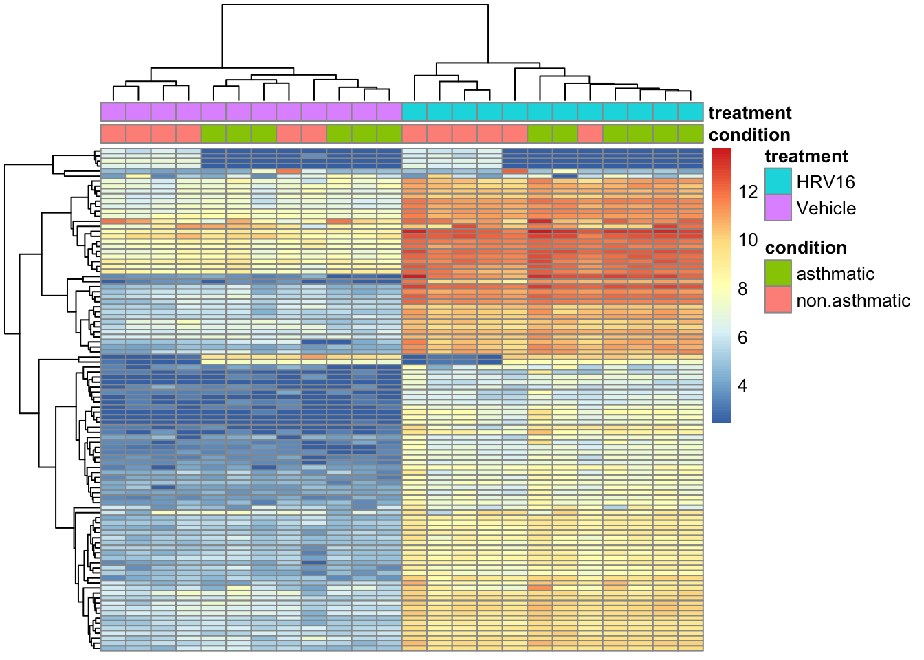
This code pull out the top of the transformed data by variance, and adds an annotation to the top of the plot.

By default the rows and columns will be clustered by Euclidean distance. See ?pheatmap for more details on this function (it’s a very detailed manual page).

library(pheatmap)
pheatmap(assay(vsd)[o,],
         annotation_col=anno_col,
         show_rownames=FALSE, 
         show_colnames=FALSE)

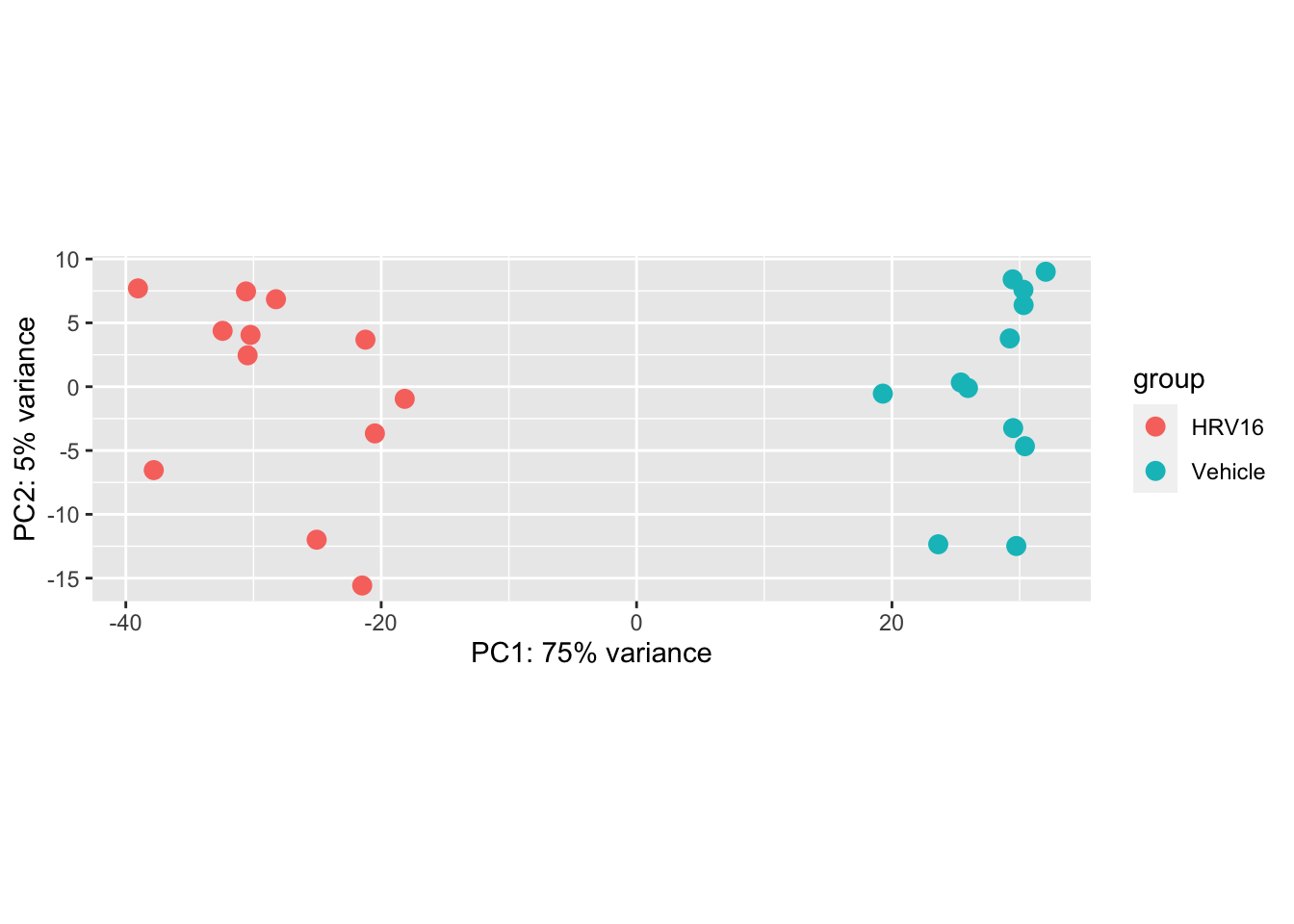
We can also easily make a PCA plot with dedicated functions:

plotPCA(vsd, intgroup="treatment")

5.10 SingleCellExperiment

An example of a class that extends the SE is SingleCellExperiment. This is a special object type for looking at single cell data.

For more details, there is a free online book “Orchestrating Single Cell Analysis With Bioconductor” produced by a group within the Bioconductor Project, with lots of example analyses: OSCA.

Here we show a quick example of how this object extends the SE.

library(SingleCellExperiment)
sce <- as(rse, "SingleCellExperiment")
sce
class: SingleCellExperiment 
dim: 58037 24 
metadata(0):
assays(1): counts
rownames(58037): ENSG00000000003.14 ENSG00000000005.5 ...
  ENSG00000283698.1 ENSG00000283699.1
rowData names(3): gene_id bp_length symbol
colnames(24): SRR1565926 SRR1565927 ... SRR1565948 SRR1565949
colData names(23): project sample ... condition treatment
reducedDimNames(0):
mainExpName: NULL
altExpNames(0):

There are special functions dedicated to scaling the samples (we will discuss this technical aspect soon):

library(scran)
Loading required package: scuttle
sce <- computeSumFactors(sce)
sizeFactors(sce)
 [1] 0.7672143 0.8205514 0.8686567 0.9479224 0.6484723 0.9815079 1.0797070
 [8] 1.0569889 1.4377886 0.9465292 1.4759422 1.2630195 0.8889808 1.0524670
[15] 0.9677885 0.8086102 0.8806503 0.8999780 0.9505805 1.0430322 1.2527967
[22] 0.9908707 0.5208294 1.4491155

Similarly, dedicated functions for transformations:

sce <- logNormCounts(sce)
assayNames(sce)
[1] "counts"    "logcounts"

And dedicated functions and new slots for reduced dimensions:

set.seed(1)
sce <- fixedPCA(sce, rank=5, subset.row=NULL)
reducedDimNames(sce)
[1] "PCA"

We can manually get at the PCs:

pca <- reducedDim(sce, "PCA")
plot(pca[,1:2])

But we can more easily use dedicated visualization functions:

library(scater)
plotReducedDim(sce, "PCA", colour_by="treatment")

5.11 Session Info

sessionInfo()
R version 4.2.2 (2022-10-31)
Platform: aarch64-apple-darwin21.6.0 (64-bit)
Running under: macOS Ventura 13.0.1

Matrix products: default
BLAS:   /opt/homebrew/Cellar/openblas/0.3.21/lib/libopenblasp-r0.3.21.dylib
LAPACK: /opt/homebrew/Cellar/r/4.2.2/lib/R/lib/libRlapack.dylib

locale:
[1] en_US.UTF-8/en_US.UTF-8/en_US.UTF-8/C/en_US.UTF-8/en_US.UTF-8

attached base packages:
[1] stats4    stats     graphics  grDevices utils     datasets  methods  
[8] base     

other attached packages:
 [1] scater_1.24.0               ggplot2_3.4.0              
 [3] scran_1.24.1                scuttle_1.6.3              
 [5] SingleCellExperiment_1.18.1 pheatmap_1.0.12            
 [7] DESeq2_1.36.0               magrittr_2.0.3             
 [9] here_1.0.1                  EnsDb.Hsapiens.v86_2.99.0  
[11] ensembldb_2.20.2            AnnotationFilter_1.20.0    
[13] GenomicFeatures_1.48.4      AnnotationDbi_1.58.0       
[15] SummarizedExperiment_1.26.1 Biobase_2.56.0             
[17] GenomicRanges_1.48.0        GenomeInfoDb_1.32.4        
[19] IRanges_2.30.1              S4Vectors_0.34.0           
[21] BiocGenerics_0.42.0         MatrixGenerics_1.8.1       
[23] matrixStats_0.63.0         

loaded via a namespace (and not attached):
  [1] BiocFileCache_2.4.0       igraph_1.3.5             
  [3] lazyeval_0.2.2            splines_4.2.2            
  [5] BiocParallel_1.30.4       digest_0.6.30            
  [7] htmltools_0.5.3           viridis_0.6.2            
  [9] fansi_1.0.3               memoise_2.0.1            
 [11] ScaledMatrix_1.4.1        cluster_2.1.4            
 [13] limma_3.52.4              Biostrings_2.64.1        
 [15] annotate_1.74.0           prettyunits_1.1.1        
 [17] colorspace_2.0-3          blob_1.2.3               
 [19] rappdirs_0.3.3            ggrepel_0.9.2            
 [21] xfun_0.35                 dplyr_1.0.10             
 [23] crayon_1.5.2              RCurl_1.98-1.9           
 [25] jsonlite_1.8.3            genefilter_1.78.0        
 [27] survival_3.4-0            glue_1.6.2               
 [29] gtable_0.3.1              zlibbioc_1.42.0          
 [31] XVector_0.36.0            DelayedArray_0.22.0      
 [33] BiocSingular_1.12.0       scales_1.2.1             
 [35] DBI_1.1.3                 edgeR_3.38.4             
 [37] Rcpp_1.0.9                viridisLite_0.4.1        
 [39] xtable_1.8-4              progress_1.2.2           
 [41] dqrng_0.3.0               bit_4.0.5                
 [43] rsvd_1.0.5                metapod_1.4.0            
 [45] htmlwidgets_1.5.4         httr_1.4.4               
 [47] RColorBrewer_1.1-3        ellipsis_0.3.2           
 [49] pkgconfig_2.0.3           XML_3.99-0.12            
 [51] farver_2.1.1              dbplyr_2.2.1             
 [53] locfit_1.5-9.6            utf8_1.2.2               
 [55] tidyselect_1.2.0          labeling_0.4.2           
 [57] rlang_1.0.6               munsell_0.5.0            
 [59] tools_4.2.2               cachem_1.0.6             
 [61] cli_3.4.1                 generics_0.1.3           
 [63] RSQLite_2.2.19            evaluate_0.18            
 [65] stringr_1.4.1             fastmap_1.1.0            
 [67] yaml_2.3.6                knitr_1.41               
 [69] bit64_4.0.5               KEGGREST_1.36.3          
 [71] sparseMatrixStats_1.8.0   xml2_1.3.3               
 [73] biomaRt_2.52.0            BiocStyle_2.24.0         
 [75] compiler_4.2.2            rstudioapi_0.14          
 [77] beeswarm_0.4.0            filelock_1.0.2           
 [79] curl_4.3.3                png_0.1-7                
 [81] tibble_3.1.8              statmod_1.4.37           
 [83] geneplotter_1.74.0        stringi_1.7.8            
 [85] lattice_0.20-45           bluster_1.6.0            
 [87] ProtGenerics_1.28.0       Matrix_1.5-3             
 [89] vctrs_0.5.1               pillar_1.8.1             
 [91] lifecycle_1.0.3           BiocManager_1.30.19      
 [93] BiocNeighbors_1.14.0      bitops_1.0-7             
 [95] irlba_2.3.5.1             rtracklayer_1.56.1       
 [97] R6_2.5.1                  BiocIO_1.6.0             
 [99] gridExtra_2.3             vipor_0.4.5              
[101] codetools_0.2-18          assertthat_0.2.1         
[103] rprojroot_2.0.3           rjson_0.2.21             
[105] withr_2.5.0               GenomicAlignments_1.32.1 
[107] Rsamtools_2.12.0          GenomeInfoDbData_1.2.8   
[109] parallel_4.2.2            hms_1.1.2                
[111] grid_4.2.2                beachmat_2.12.0          
[113] rmarkdown_2.18            DelayedMatrixStats_1.18.2
[115] ggbeeswarm_0.6.0          restfulr_0.0.15