3 Tidyverse and data viz

library(tidyverse)

“Happy families are all alike; every unhappy family is unhappy in its own way.” —- Leo Tolstoy

“Tidy datasets are all alike, but every messy dataset is messy in its own way.” —- Hadley Wickham

3.1 Learning objectives

Know difference between relative vs absolute paths
Use modern R packages (readr) for reading and writing data in R
Understand the advantages of a tibble and data.frame data objects in R
Learn about the dplyr R package to manage data frames
Recognize the key verbs to manage data frames in dplyr
Use the “pipe” operator to combine verbs together
Be able to build up layers of graphics using ggplot()

3.2 Reading and writing data

Here, we introduce ays to read and write data (e.g. .txt and .csv files) using base R functions as well as more modern R packages, such as readr, which is typically 10x faster than base R.

3.2.1 Relative paths

When you open up a .Rproj file, RStudio changes the path (location on your computer) to the .Rproj location.

After opening up a .Rproj file, you can test this by

getwd()

When you open up someone else’s R code or analysis, you might also see the

setwd()

function being used which explicitly tells R to change the absolute path or absolute location of which directory to move into.

For example, say I want to clone a GitHub repo from Roger, which has 100 R script files, and in every one of those files at the top is:

setwd("C:\Users\Roger\path\only\that\Roger\has")

The problem is, if I want to use his code, I will need to go and hand-edit every single one of those paths (C:\Users\Roger\path\only\that\Roger\has) to the path that I want to use on my computer or wherever I saved the folder on my computer (e.g. /Users/Stephanie/Documents/path/only/I/have).

This is an unsustainable practice.
I can go in and manually edit the path, but this assumes I know how to set a working directory. Not everyone does.

So instead of absolute paths:

setwd("/Users/jtleek/data")
setwd("~/Desktop/files/data")
setwd("C:\\Users\\Michelle\\Downloads")

A better idea is to use relative paths with the here R package.

It will recognize the top-level directory of a Git repo and supports building all paths relative to that.
For more on project-oriented workflow suggestions, read this post from Jenny Bryan.

3.2.2 The `here` package

Let’s try using the here package.

library(here)

here() starts at /Users/stephaniehicks/Documents/github/teaching/cshlcg2022

here::here()

[1] "/Users/stephaniehicks/Documents/github/teaching/cshlcg2022"

This function creates a path unique to my computer, but will also be unique to yours.

list.files(here::here())

 [1] "_book"                    "_freeze"                 
 [3] "_quarto.yml"              "cover.png"               
 [5] "cshlcg2022.Rproj"         "data"                    
 [7] "exercises-01.qmd"         "exercises-02.qmd"        
 [9] "exercises-03.qmd"         "exercises-04.qmd"        
[11] "figures"                  "index.qmd"               
[13] "intro-to-bioc.qmd"        "intro-to-r.qmd"          
[15] "intro-to-single-cell.qmd" "references.bib"          
[17] "references.qmd"           "reproducible-res.qmd"    
[19] "tidyverse.qmd"            "tidyverse.rmarkdown"

list.files(here("data"))

[1] "asthma.rda"         "chicago.rds"        "spotify_songs.RDS" 
[4] "team_standings.csv"

list.files(here("data", "team_standings.csv"))

character(0)

Now we see that using the here::here() function is a relative path (relative to the .Rproj file in our cshlcg2022 folder.

Next, let’s use the here package to read in some data with the readr package.

3.2.3 The `readr` package

The readr package is recently developed by posit (formerly RStudio) to deal with reading in large flat files quickly. The package provides replacements for functions like read.table() and read.csv(). The analogous functions in readr are read_table() and read_csv().

These functions are often much faster than their base R analogues and provide a few other nice features such as progress meters.

For example, the package includes a variety of functions in the read_*() family that allow you to read in data from different formats of flat files. The following table gives a guide to several functions in the read_*() family.

`readr` function	Use
`read_csv()`	Reads comma-separated file
`read_csv2()`	Reads semicolon-separated file
`read_tsv()`	Reads tab-separated file
`read_delim()`	General function for reading delimited files
`read_fwf()`	Reads fixed width files
`read_log()`	Reads log files

A typical call to read_csv() will look as follows.

library(readr)
teams <- read_csv(here("data", "team_standings.csv"))

Rows: 32 Columns: 2
── Column specification ────────────────────────────────────────────────────────
Delimiter: ","
chr (1): Team
dbl (1): Standing

ℹ Use `spec()` to retrieve the full column specification for this data.
ℹ Specify the column types or set `show_col_types = FALSE` to quiet this message.

teams

# A tibble: 32 × 2
   Standing Team       
      <dbl> <chr>      
 1        1 Spain      
 2        2 Netherlands
 3        3 Germany    
 4        4 Uruguay    
 5        5 Argentina  
 6        6 Brazil     
 7        7 Ghana      
 8        8 Paraguay   
 9        9 Japan      
10       10 Chile      
# … with 22 more rows

3.3 Data frames and tibbles

The data frame (or data.frame) is a key data structure in statistics and in R.

The basic structure of a data frame is that there is one observation per row and each column represents a variable, a measure, feature, or characteristic of that observation.

Given the importance of managing data frames, it is important that we have good tools for dealing with them.

For example, operations like filtering rows, re-ordering rows, and selecting columns, can often be tedious operations in R whose syntax is not very intuitive. The dplyr package in the tidyverse is designed to mitigate a lot of these problems and to provide a highly optimized set of routines specifically for dealing with data frames.

3.3.1 Tibbles

Another type of data structure that we need to discuss is called the tibble! It’s best to think of tibbles as an updated and stylish version of the data.frame.

Tibbles are what tidyverse packages work with most seamlessly. Now, that does not mean tidyverse packages require tibbles.

In fact, they still work with data.frames, but the more you work with tidyverse and tidyverse-adjacent packages, the more you will see the advantages of using tibbles.

Before we go any further, tibbles are data frames, but they have some new bells and whistles to make your life easier.

3.3.2 How tibbles differ from `data.frame`

There are a number of differences between tibbles and data.frames.

Note

To see a full vignette about tibbles and how they differ from data.frame, you will want to execute vignette("tibble") and read through that vignette.

We will summarize some of the most important points here:

Input type remains unchanged - data.frame is notorious for treating strings as factors; this will not happen with tibbles
Variable names remain unchanged - In base R, creating data.frames will remove spaces from names, converting them to periods or add “x” before numeric column names. Creating tibbles will not change variable (column) names.
There are no row.names() for a tibble - Tidy data requires that variables be stored in a consistent way, removing the need for row names.
Tibbles print first ten rows and columns that fit on one screen - Printing a tibble to screen will never print the entire huge data frame out. By default, it just shows what fits to your screen.

3.3.3 `as_tibble()`

Since many packages use the historical data.frame from base R, you will often find yourself in the situation that you have a data.frame and want to convert that data.frame to a tibble.

To do so, the as_tibble() function is exactly what you are looking for.

For the example, here we use a dataset (chicago.rds) containing air pollution and temperature data for the city of Chicago in the U.S.

The dataset is available in the /data repository. You can load the data into R using the readRDS() function.

library(here)
chicago <- readRDS(here("data", "chicago.rds"))

You can see some basic characteristics of the dataset with the dim() and str() functions.

dim(chicago)

[1] 6940    8

str(chicago)

'data.frame':   6940 obs. of  8 variables:
 $ city      : chr  "chic" "chic" "chic" "chic" ...
 $ tmpd      : num  31.5 33 33 29 32 40 34.5 29 26.5 32.5 ...
 $ dptp      : num  31.5 29.9 27.4 28.6 28.9 ...
 $ date      : Date, format: "1987-01-01" "1987-01-02" ...
 $ pm25tmean2: num  NA NA NA NA NA NA NA NA NA NA ...
 $ pm10tmean2: num  34 NA 34.2 47 NA ...
 $ o3tmean2  : num  4.25 3.3 3.33 4.38 4.75 ...
 $ no2tmean2 : num  20 23.2 23.8 30.4 30.3 ...

We see this data structure is a data.frame with 6940 observations and 8 variables.

To convert this data.frame to a tibble you would use the following:

str(as_tibble(chicago))

tibble [6,940 × 8] (S3: tbl_df/tbl/data.frame)
 $ city      : chr [1:6940] "chic" "chic" "chic" "chic" ...
 $ tmpd      : num [1:6940] 31.5 33 33 29 32 40 34.5 29 26.5 32.5 ...
 $ dptp      : num [1:6940] 31.5 29.9 27.4 28.6 28.9 ...
 $ date      : Date[1:6940], format: "1987-01-01" "1987-01-02" ...
 $ pm25tmean2: num [1:6940] NA NA NA NA NA NA NA NA NA NA ...
 $ pm10tmean2: num [1:6940] 34 NA 34.2 47 NA ...
 $ o3tmean2  : num [1:6940] 4.25 3.3 3.33 4.38 4.75 ...
 $ no2tmean2 : num [1:6940] 20 23.2 23.8 30.4 30.3 ...

3.4 The `dplyr` package

The dplyr package was developed by Posit (formely RStudio) and is an optimized and distilled version of the older plyr package for data manipulation or wrangling.

The dplyr package does not provide any “new” functionality to R per se, in the sense that everything dplyr does could already be done with base R, but it greatly simplifies existing functionality in R.

One important contribution of the dplyr package is that it provides a “grammar” (in particular, verbs) for data manipulation and for operating on data frames.

With this grammar, you can sensibly communicate what it is that you are doing to a data frame that other people can understand (assuming they also know the grammar). This is useful because it provides an abstraction for data manipulation that previously did not exist.

Another useful contribution is that the dplyr functions are very fast, as many key operations are coded in C++.

3.4.1 `dplyr` grammar

Some of the key “verbs” provided by the dplyr package are

select(): return a subset of the columns of a data frame, using a flexible notation
filter(): extract a subset of rows from a data frame based on logical conditions
arrange(): reorder rows of a data frame
rename(): rename variables in a data frame
mutate(): add new variables/columns or transform existing variables
summarise() / summarize(): generate summary statistics of different variables in the data frame, possibly within strata
%>%: the “pipe” operator is used to connect multiple verb actions together into a pipeline

Note

The dplyr package as a number of its own data types that it takes advantage of.

For example, there is a handy print() method that prevents you from printing a lot of data to the console. Most of the time, these additional data types are transparent to the user and do not need to be worried about.

3.4.2 `dplyr` installation

The dplyr package is installed when you install and load the tidyverse meta-package.

library(tidyverse)

You may get some warnings when the package is loaded because there are functions in the dplyr package that have the same name as functions in other packages. For now you can ignore the warnings.

3.5 `dplyr` functions

All of the functions that we will discuss here will have a few common characteristics. In particular,

The first argument is a data frame type object.
The subsequent arguments describe what to do with the data frame specified in the first argument, and you can refer to columns in the data frame directly (without using the $ operator, just use the column names).
The return result of a function is a new data frame.
Data frames must be properly formatted and annotated for this to all be useful. In particular, the data must be tidy. In short, there should be one observation per row, and each column should represent a feature or characteristic of that observation.

3.5.1 `select()`

We will continue to use the chicago dataset containing air pollution and temperature data.

chicago <- as_tibble(chicago)
str(chicago)

tibble [6,940 × 8] (S3: tbl_df/tbl/data.frame)
 $ city      : chr [1:6940] "chic" "chic" "chic" "chic" ...
 $ tmpd      : num [1:6940] 31.5 33 33 29 32 40 34.5 29 26.5 32.5 ...
 $ dptp      : num [1:6940] 31.5 29.9 27.4 28.6 28.9 ...
 $ date      : Date[1:6940], format: "1987-01-01" "1987-01-02" ...
 $ pm25tmean2: num [1:6940] NA NA NA NA NA NA NA NA NA NA ...
 $ pm10tmean2: num [1:6940] 34 NA 34.2 47 NA ...
 $ o3tmean2  : num [1:6940] 4.25 3.3 3.33 4.38 4.75 ...
 $ no2tmean2 : num [1:6940] 20 23.2 23.8 30.4 30.3 ...

The select() function can be used to select columns of a data frame that you want to focus on.

Example

Suppose we wanted to take the first 3 columns only. There are a few ways to do this.

We could for example use numerical indices:

names(chicago)[1:3]

[1] "city" "tmpd" "dptp"

But we can also use the names directly:

subset <- select(chicago, city:dptp)
head(subset)

# A tibble: 6 × 3
  city   tmpd  dptp
  <chr> <dbl> <dbl>
1 chic   31.5  31.5
2 chic   33    29.9
3 chic   33    27.4
4 chic   29    28.6
5 chic   32    28.9
6 chic   40    35.1

Note

The : normally cannot be used with names or strings, but inside the select() function you can use it to specify a range of variable names.

You can also omit variables using the select() function by using the negative sign. With select() you can do

select(chicago, -(city:dptp))

which indicates that we should include every variable except the variables city through dptp. The equivalent code in base R would be

i <- match("city", names(chicago))
j <- match("dptp", names(chicago))
head(chicago[, -(i:j)])

Not super intuitive, right?

The select() function also allows a special syntax that allows you to specify variable names based on patterns. So, for example, if you wanted to keep every variable that ends with a “2”, we could do

subset <- select(chicago, ends_with("2"))
str(subset)

tibble [6,940 × 4] (S3: tbl_df/tbl/data.frame)
 $ pm25tmean2: num [1:6940] NA NA NA NA NA NA NA NA NA NA ...
 $ pm10tmean2: num [1:6940] 34 NA 34.2 47 NA ...
 $ o3tmean2  : num [1:6940] 4.25 3.3 3.33 4.38 4.75 ...
 $ no2tmean2 : num [1:6940] 20 23.2 23.8 30.4 30.3 ...

Or if we wanted to keep every variable that starts with a “d”, we could do

subset <- select(chicago, starts_with("d"))
str(subset)

tibble [6,940 × 2] (S3: tbl_df/tbl/data.frame)
 $ dptp: num [1:6940] 31.5 29.9 27.4 28.6 28.9 ...
 $ date: Date[1:6940], format: "1987-01-01" "1987-01-02" ...

You can also use more general regular expressions if necessary. See the help page (?select) for more details.

3.5.2 `filter()`

The filter() function is used to extract subsets of rows from a data frame. This function is similar to the existing subset() function in R but is quite a bit faster in my experience.

Example

Suppose we wanted to extract the rows of the chicago data frame where the levels of PM2.5 are greater than 30 (which is a reasonably high level), we could do

chic.f <- filter(chicago, pm25tmean2 > 30)
str(chic.f)

tibble [194 × 8] (S3: tbl_df/tbl/data.frame)
 $ city      : chr [1:194] "chic" "chic" "chic" "chic" ...
 $ tmpd      : num [1:194] 23 28 55 59 57 57 75 61 73 78 ...
 $ dptp      : num [1:194] 21.9 25.8 51.3 53.7 52 56 65.8 59 60.3 67.1 ...
 $ date      : Date[1:194], format: "1998-01-17" "1998-01-23" ...
 $ pm25tmean2: num [1:194] 38.1 34 39.4 35.4 33.3 ...
 $ pm10tmean2: num [1:194] 32.5 38.7 34 28.5 35 ...
 $ o3tmean2  : num [1:194] 3.18 1.75 10.79 14.3 20.66 ...
 $ no2tmean2 : num [1:194] 25.3 29.4 25.3 31.4 26.8 ...

You can see that there are now only 194 rows in the data frame and the distribution of the pm25tmean2 values is.

summary(chic.f$pm25tmean2)

   Min. 1st Qu.  Median    Mean 3rd Qu.    Max. 
  30.05   32.12   35.04   36.63   39.53   61.50

We can place an arbitrarily complex logical sequence inside of filter(), so we could for example extract the rows where PM2.5 is greater than 30 and temperature is greater than 80 degrees Fahrenheit.

chic.f <- filter(chicago, pm25tmean2 > 30 & tmpd > 80)
select(chic.f, date, tmpd, pm25tmean2)

# A tibble: 17 × 3
   date        tmpd pm25tmean2
   <date>     <dbl>      <dbl>
 1 1998-08-23    81       39.6
 2 1998-09-06    81       31.5
 3 2001-07-20    82       32.3
 4 2001-08-01    84       43.7
 5 2001-08-08    85       38.8
 6 2001-08-09    84       38.2
 7 2002-06-20    82       33  
 8 2002-06-23    82       42.5
 9 2002-07-08    81       33.1
10 2002-07-18    82       38.8
11 2003-06-25    82       33.9
12 2003-07-04    84       32.9
13 2005-06-24    86       31.9
14 2005-06-27    82       51.5
15 2005-06-28    85       31.2
16 2005-07-17    84       32.7
17 2005-08-03    84       37.9

Now there are only 17 observations where both of those conditions are met.

Other logical operators you should be aware of include:

Operator	Meaning	Example
`==`	Equals	`city == chic`
`!=`	Does not equal	`city != chic`
`>`	Greater than	`tmpd > 32.0`
`>=`	Greater than or equal to	`tmpd >- 32.0`
`<`	Less than	`tmpd < 32.0`
`<=`	Less than or equal to	`tmpd <= 32.0`
`%in%`	Included in	`city %in% c("chic", "bmore")`
`is.na()`	Is a missing value	`is.na(pm10tmean2)`

Note: If you are ever unsure of how to write a logical statement, but know how to write its opposite, you can use the ! operator to negate the whole statement.

A common use of this is to identify observations with non-missing data (e.g., !(is.na(pm10tmean2))).

3.5.3 `arrange()`

The arrange() function is used to reorder rows of a data frame according to one of the variables/columns. Reordering rows of a data frame (while preserving corresponding order of other columns) is normally a pain to do in R. The arrange() function simplifies the process quite a bit.

Here we can order the rows of the data frame by date, so that the first row is the earliest (oldest) observation and the last row is the latest (most recent) observation.

chicago <- arrange(chicago, date)

We can now check the first few rows

head(select(chicago, date, pm25tmean2), 3)

# A tibble: 3 × 2
  date       pm25tmean2
  <date>          <dbl>
1 1987-01-01         NA
2 1987-01-02         NA
3 1987-01-03         NA

and the last few rows.

tail(select(chicago, date, pm25tmean2), 3)

# A tibble: 3 × 2
  date       pm25tmean2
  <date>          <dbl>
1 2005-12-29       7.45
2 2005-12-30      15.1 
3 2005-12-31      15

Columns can be arranged in descending order too by useing the special desc() operator.

chicago <- arrange(chicago, desc(date))

Looking at the first three and last three rows shows the dates in descending order.

head(select(chicago, date, pm25tmean2), 3)

# A tibble: 3 × 2
  date       pm25tmean2
  <date>          <dbl>
1 2005-12-31      15   
2 2005-12-30      15.1 
3 2005-12-29       7.45

tail(select(chicago, date, pm25tmean2), 3)

# A tibble: 3 × 2
  date       pm25tmean2
  <date>          <dbl>
1 1987-01-03         NA
2 1987-01-02         NA
3 1987-01-01         NA

3.5.4 `rename()`

Renaming a variable in a data frame in R is surprisingly hard to do! The rename() function is designed to make this process easier.

Here you can see the names of the first five variables in the chicago data frame.

head(chicago[, 1:5], 3)

# A tibble: 3 × 5
  city   tmpd  dptp date       pm25tmean2
  <chr> <dbl> <dbl> <date>          <dbl>
1 chic     35  30.1 2005-12-31      15   
2 chic     36  31   2005-12-30      15.1 
3 chic     35  29.4 2005-12-29       7.45

The dptp column is supposed to represent the dew point temperature and the pm25tmean2 column provides the PM2.5 data.

However, these names are pretty obscure or awkward and probably be renamed to something more sensible.

chicago <- rename(chicago, dewpoint = dptp, pm25 = pm25tmean2)
head(chicago[, 1:5], 3)

# A tibble: 3 × 5
  city   tmpd dewpoint date        pm25
  <chr> <dbl>    <dbl> <date>     <dbl>
1 chic     35     30.1 2005-12-31 15   
2 chic     36     31   2005-12-30 15.1 
3 chic     35     29.4 2005-12-29  7.45

The syntax inside the rename() function is to have the new name on the left-hand side of the = sign and the old name on the right-hand side.

3.5.5 `mutate()`

The mutate() function exists to compute transformations of variables in a data frame. Often, you want to create new variables that are derived from existing variables and mutate() provides a clean interface for doing that.

For example, with air pollution data, we often want to detrend the data by subtracting the mean from the data.

That way we can look at whether a given day’s air pollution level is higher than or less than average (as opposed to looking at its absolute level).

Here, we create a pm25detrend variable that subtracts the mean from the pm25 variable.

chicago <- mutate(chicago, pm25detrend = pm25 - mean(pm25, na.rm = TRUE))
head(chicago)

# A tibble: 6 × 9
  city   tmpd dewpoint date        pm25 pm10tmean2 o3tmean2 no2tmean2 pm25detr…¹
  <chr> <dbl>    <dbl> <date>     <dbl>      <dbl>    <dbl>     <dbl>      <dbl>
1 chic     35     30.1 2005-12-31 15          23.5     2.53      13.2      -1.23
2 chic     36     31   2005-12-30 15.1        19.2     3.03      22.8      -1.17
3 chic     35     29.4 2005-12-29  7.45       23.5     6.79      20.0      -8.78
4 chic     37     34.5 2005-12-28 17.8        27.5     3.26      19.3       1.52
5 chic     40     33.6 2005-12-27 23.6        27       4.47      23.5       7.33
6 chic     35     29.6 2005-12-26  8.4         8.5    14.0       16.8      -7.83
# … with abbreviated variable name ¹pm25detrend

There is also the related transmute() function, which does the same thing as mutate() but then drops all non-transformed variables.

Here, we de-trend the PM10 and ozone (O3) variables.

head(transmute(chicago, 
               pm10detrend = pm10tmean2 - mean(pm10tmean2, na.rm = TRUE),
               o3detrend = o3tmean2 - mean(o3tmean2, na.rm = TRUE)))

# A tibble: 6 × 2
  pm10detrend o3detrend
        <dbl>     <dbl>
1      -10.4     -16.9 
2      -14.7     -16.4 
3      -10.4     -12.6 
4       -6.40    -16.2 
5       -6.90    -15.0 
6      -25.4      -5.39

Note that there are only two columns in the transmuted data frame.

3.5.6 `group_by()`

The group_by() function is used to generate summary statistics from the data frame within strata defined by a variable.

For example, in this air pollution dataset, you might want to know what the average annual level of PM2.5 is?

So the stratum is the year, and that is something we can derive from the date variable.

In conjunction with the group_by() function, we often use the summarize() function (or summarise() for some parts of the world).

Note: The general operation here is a combination of

Splitting a data frame into separate pieces defined by a variable or group of variables (group_by())
Then, applying a summary function across those subsets (summarize())

Example

First, we can create a year variable using as.POSIXlt().

chicago <- mutate(chicago, year = as.POSIXlt(date)$year + 1900)

Now we can create a separate data frame that splits the original data frame by year.

years <- group_by(chicago, year)

Finally, we compute summary statistics for each year in the data frame with the summarize() function.

summarize(years, 
          pm25 = mean(pm25, na.rm = TRUE), 
          o3 = max(o3tmean2, na.rm = TRUE), 
          no2 = median(no2tmean2, na.rm = TRUE))

# A tibble: 19 × 4
    year  pm25    o3   no2
   <dbl> <dbl> <dbl> <dbl>
 1  1987 NaN    63.0  23.5
 2  1988 NaN    61.7  24.5
 3  1989 NaN    59.7  26.1
 4  1990 NaN    52.2  22.6
 5  1991 NaN    63.1  21.4
 6  1992 NaN    50.8  24.8
 7  1993 NaN    44.3  25.8
 8  1994 NaN    52.2  28.5
 9  1995 NaN    66.6  27.3
10  1996 NaN    58.4  26.4
11  1997 NaN    56.5  25.5
12  1998  18.3  50.7  24.6
13  1999  18.5  57.5  24.7
14  2000  16.9  55.8  23.5
15  2001  16.9  51.8  25.1
16  2002  15.3  54.9  22.7
17  2003  15.2  56.2  24.6
18  2004  14.6  44.5  23.4
19  2005  16.2  58.8  22.6

summarize() returns a data frame with year as the first column, and then the annual summary statistics of pm25, o3, and no2.

3.5.7 `%>%`

The pipeline operator %>% is very handy for stringing together multiple dplyr functions in a sequence of operations.

Notice above that every time we wanted to apply more than one function, the sequence gets buried in a sequence of nested function calls that is difficult to read, i.e.

third(second(first(x)))

This nesting is not a natural way to think about a sequence of operations.

The %>% operator allows you to string operations in a left-to-right fashion, i.e.

first(x) %>% second %>% third

Example

Take the example that we just did in the last section, but here use the pipe operator in a single expression.

mutate(chicago, year = as.POSIXlt(date)$year + 1900) %>%    
        group_by(year) %>% 
        summarize(years, pm25 = mean(pm25, na.rm = TRUE), 
          o3 = max(o3tmean2, na.rm = TRUE), 
          no2 = median(no2tmean2, na.rm = TRUE))

`summarise()` has grouped output by 'year'. You can override using the
`.groups` argument.

# A tibble: 131,860 × 12
# Groups:   year [19]
    year city   tmpd dewpoint date        pm25 pm10tme…¹ o3tme…² no2tm…³ pm25d…⁴
   <dbl> <chr> <dbl>    <dbl> <date>     <dbl>     <dbl>   <dbl>   <dbl>   <dbl>
 1  2005 chic     35     30.1 2005-12-31  16.2      23.5    2.53    13.2   -1.23
 2  2005 chic     36     31   2005-12-30  16.2      19.2    3.03    22.8   -1.17
 3  2005 chic     35     29.4 2005-12-29  16.2      23.5    6.79    20.0   -8.78
 4  2005 chic     37     34.5 2005-12-28  16.2      27.5    3.26    19.3    1.52
 5  2005 chic     40     33.6 2005-12-27  16.2      27      4.47    23.5    7.33
 6  2005 chic     35     29.6 2005-12-26  16.2       8.5   14.0     16.8   -7.83
 7  2005 chic     35     32.1 2005-12-25  16.2       8     14.4     13.8   -9.53
 8  2005 chic     37     35.2 2005-12-24  16.2      25.2    1.77    32.0   14.5 
 9  2005 chic     41     32.6 2005-12-23  16.2      34.5    6.91    29.1   16.7 
10  2005 chic     22     23.3 2005-12-22  16.2      42.5    5.39    33.7   20.4 
# … with 131,850 more rows, 2 more variables: o3 <dbl>, no2 <dbl>, and
#   abbreviated variable names ¹pm10tmean2, ²o3tmean2, ³no2tmean2, ⁴pm25detrend

Note

In the above code, I pass the chicago data frame to the first call to mutate(), but then afterwards I do not have to pass the first argument to group_by() or summarize().

Once you travel down the pipeline with %>%, the first argument is taken to be the output of the previous element in the pipeline.

3.5.8 `slice_*()`

The slice_sample() function of the dplyr package will allow you to see a sample of random rows in random order.

The number of rows to show is specified by the n argument.

This can be useful if you do not want to print the entire tibble, but you want to get a greater sense of the values.
This is a good option for data analysis reports, where printing the entire tibble would not be appropriate if the tibble is quite large.

Example

slice_sample(chicago, n = 10)

# A tibble: 10 × 10
   city   tmpd dewpoint date        pm25 pm10tme…¹ o3tme…² no2tm…³ pm25d…⁴  year
   <chr> <dbl>    <dbl> <date>     <dbl>     <dbl>   <dbl>   <dbl>   <dbl> <dbl>
 1 chic   35       24.8 1994-11-26  NA        20.5   18.1     17.4   NA     1994
 2 chic   32       30   1993-02-07  NA        26.5    6.81    21.5   NA     1993
 3 chic   70       60.3 2004-09-01  NA        47.5   25.5     31.7   NA     2004
 4 chic   53.5     38.5 1990-09-24  NA        34     16.9     24.9   NA     1990
 5 chic   62.5     44.2 1990-05-28  NA        28     40.8     14.2   NA     1990
 6 chic   58       48.4 1998-10-15  14.8      26.5    7.40    27.1   -1.43  1998
 7 chic   40.5     37.2 1996-04-29  NA        14     21.0     23.6   NA     1996
 8 chic   38       29.2 1987-11-18  NA        NA     10.3     15.7   NA     1987
 9 chic   77       65.5 1998-07-18  NA        52.5   32.9     31.4   NA     1998
10 chic   79.5     56.8 1988-07-05  NA        NA     57.7     51.4   NA     1988
# … with abbreviated variable names ¹pm10tmean2, ²o3tmean2, ³no2tmean2,
#   ⁴pm25detrend

You can also use slice_head() or slice_tail() to take a look at the top rows or bottom rows of your tibble. Again the number of rows can be specified with the n argument.

This will show the first 5 rows.

slice_head(chicago, n = 5)

# A tibble: 5 × 10
  city   tmpd dewpoint date        pm25 pm10tmean2 o3tme…¹ no2tm…² pm25d…³  year
  <chr> <dbl>    <dbl> <date>     <dbl>      <dbl>   <dbl>   <dbl>   <dbl> <dbl>
1 chic     35     30.1 2005-12-31 15          23.5    2.53    13.2   -1.23  2005
2 chic     36     31   2005-12-30 15.1        19.2    3.03    22.8   -1.17  2005
3 chic     35     29.4 2005-12-29  7.45       23.5    6.79    20.0   -8.78  2005
4 chic     37     34.5 2005-12-28 17.8        27.5    3.26    19.3    1.52  2005
5 chic     40     33.6 2005-12-27 23.6        27      4.47    23.5    7.33  2005
# … with abbreviated variable names ¹o3tmean2, ²no2tmean2, ³pm25detrend

This will show the last 5 rows.

slice_tail(chicago, n = 5)

# A tibble: 5 × 10
  city   tmpd dewpoint date        pm25 pm10tmean2 o3tme…¹ no2tm…² pm25d…³  year
  <chr> <dbl>    <dbl> <date>     <dbl>      <dbl>   <dbl>   <dbl>   <dbl> <dbl>
1 chic   32       28.9 1987-01-05    NA       NA      4.75    30.3      NA  1987
2 chic   29       28.6 1987-01-04    NA       47      4.38    30.4      NA  1987
3 chic   33       27.4 1987-01-03    NA       34.2    3.33    23.8      NA  1987
4 chic   33       29.9 1987-01-02    NA       NA      3.30    23.2      NA  1987
5 chic   31.5     31.5 1987-01-01    NA       34      4.25    20.0      NA  1987
# … with abbreviated variable names ¹o3tmean2, ²no2tmean2, ³pm25detrend

3.6 The ggplot2 Plotting System

In this section, we will get into a little more of the nitty gritty of how ggplot2 builds plots and how you can customize various aspects of any plot.

3.6.1 Basic components of a ggplot2 plot

A ggplot2 plot consists of a number of key components.

A data frame: stores all of the data that will be displayed on the plot
aesthetic mappings: describe how data are mapped to color, size, shape, location
geoms: geometric objects like points, lines, shapes
facets: describes how conditional/panel plots should be constructed
stats: statistical transformations like binning, quantiles, smoothing
scales: what scale an aesthetic map uses (example: left-handed = red, right-handed = blue)
coordinate system: describes the system in which the locations of the geoms will be drawn

It is essential to organize your data into a data frame before you start with ggplot2 (and all the appropriate metadata so that your data frame is self-describing and your plots will be self-documenting).

When building plots in ggplot2 (rather than using qplot()), the “artist’s palette” model may be the closest analogy.

Essentially, you start with some raw data, and then you gradually add bits and pieces to it to create a plot.

Note

Plots are built up in layers, with the typically ordering being

Plot the data
Overlay a summary
Add metadata and annotation

For quick exploratory plots you may not get past step 1.

3.7 Building up in layers

First, we can create a ggplot object that stores the dataset and the basic aesthetics for mapping the x- and y-coordinates for the plot.

3.7.1 `palmerpenguins` dataset

Here we will use the palmerpenguins dataset. These data contain observations for 344 penguins. There are 3 different species of penguins in this dataset, collected from 3 islands in the Palmer Archipelago, Antarctica.

[Source: Artwork by Allison Horst]

library(palmerpenguins)

glimpse(penguins)

Rows: 344
Columns: 8
$ species           <fct> Adelie, Adelie, Adelie, Adelie, Adelie, Adelie, Adel…
$ island            <fct> Torgersen, Torgersen, Torgersen, Torgersen, Torgerse…
$ bill_length_mm    <dbl> 39.1, 39.5, 40.3, NA, 36.7, 39.3, 38.9, 39.2, 34.1, …
$ bill_depth_mm     <dbl> 18.7, 17.4, 18.0, NA, 19.3, 20.6, 17.8, 19.6, 18.1, …
$ flipper_length_mm <int> 181, 186, 195, NA, 193, 190, 181, 195, 193, 190, 186…
$ body_mass_g       <int> 3750, 3800, 3250, NA, 3450, 3650, 3625, 4675, 3475, …
$ sex               <fct> male, female, female, NA, female, male, female, male…
$ year              <int> 2007, 2007, 2007, 2007, 2007, 2007, 2007, 2007, 2007…

If we wanted to count the number of penguins for each of the three species, we can use the count() function in dplyr:

penguins %>% 
  count(species)

# A tibble: 3 × 2
  species       n
  <fct>     <int>
1 Adelie      152
2 Chinstrap    68
3 Gentoo      124

For example, we see there are a total of 152 Adelie penguins in the palmerpenguins dataset.

g <- ggplot(penguins, aes(x = flipper_length_mm, 
                          y = bill_length_mm))
summary(g)

data: species, island, bill_length_mm, bill_depth_mm,
  flipper_length_mm, body_mass_g, sex, year [344x8]
mapping:  x = ~flipper_length_mm, y = ~bill_length_mm
faceting: <ggproto object: Class FacetNull, Facet, gg>
    compute_layout: function
    draw_back: function
    draw_front: function
    draw_labels: function
    draw_panels: function
    finish_data: function
    init_scales: function
    map_data: function
    params: list
    setup_data: function
    setup_params: function
    shrink: TRUE
    train_scales: function
    vars: function
    super:  <ggproto object: Class FacetNull, Facet, gg>

class(g)

[1] "gg"     "ggplot"

You can see above that the object g contains the dataset penguins and the mappings.

Now, normally if you were to print() a ggplot object a plot would appear on the plot device, however, our object g actually does not contain enough information to make a plot yet.

g <- penguins %>% 
      ggplot(aes(x = flipper_length_mm, 
                 y = bill_length_mm))
print(g)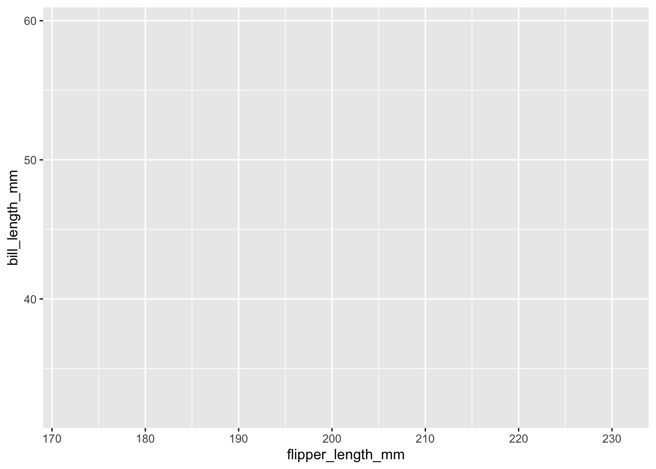

3.7.2 First plot with point layer

To make a scatter plot, we need add at least one geom, such as points.

Here, we add the geom_point() function to create a traditional scatter plot.

g <- penguins %>% 
      ggplot(aes(x = flipper_length_mm, 
                 y = bill_length_mm))
g + geom_point()

Warning: Removed 2 rows containing missing values (`geom_point()`).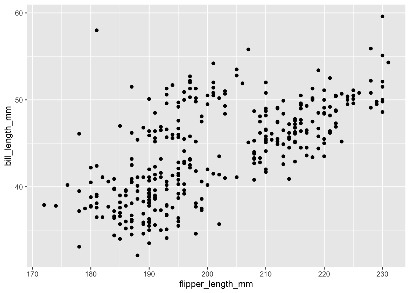

How does ggplot know what points to plot? In this case, it can grab them from the data frame penguins that served as the input into the ggplot() function.

3.7.3 Adding more layers

3.7.3.1 smooth

Because the data appear rather noisy, it might be better if we added a smoother on top of the points to see if there is a trend in the data with PM2.5.

g + 
  geom_point() + 
  geom_smooth()

Warning: Removed 2 rows containing non-finite values (`stat_smooth()`).

Warning: Removed 2 rows containing missing values (`geom_point()`).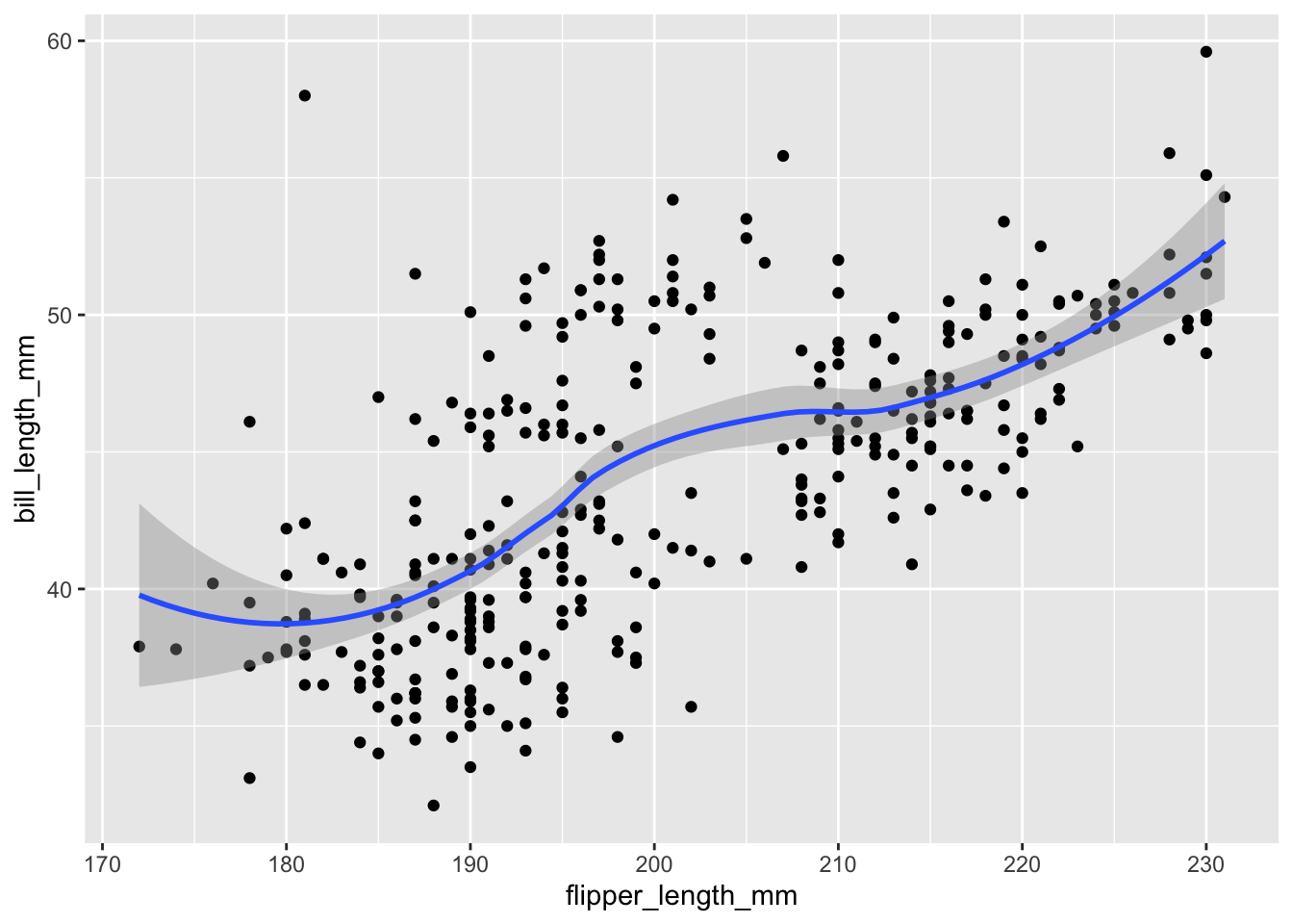

The default smoother is a loess smoother, which is flexible and nonparametric but might be too flexible for our purposes. Perhaps we’d prefer a simple linear regression line to highlight any first order trends. We can do this by specifying method = "lm" to geom_smooth().

g + 
  geom_point() + 
  geom_smooth(method = "lm")

Warning: Removed 2 rows containing non-finite values (`stat_smooth()`).

Warning: Removed 2 rows containing missing values (`geom_point()`).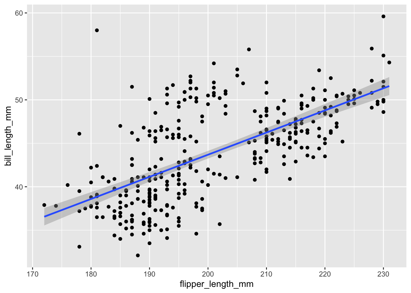

Here, we can see there appears to be a increasing trend.

We can color the points by species and a smoother by adding a linear regression.

penguins %>% 
  ggplot(aes(x = flipper_length_mm, 
             y = bill_length_mm, 
             color = species)) + 
  geom_point() + 
  geom_smooth(method = "lm")

Warning: Removed 2 rows containing non-finite values (`stat_smooth()`).

Warning: Removed 2 rows containing missing values (`geom_point()`).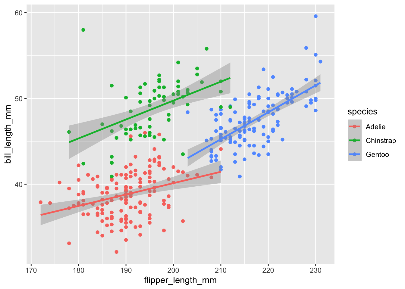

3.7.3.2 facets

We can also stratify the scatter plot by another variable (e.g. sex) by adding a facet_grid() or facet_wrap() function.

penguins %>% 
  filter(!is.na(sex)) %>% 
  ggplot(aes(x = flipper_length_mm, 
             y = bill_length_mm, 
             color = species)) + 
  geom_point() + 
  geom_smooth(method = "lm") + 
  facet_grid(.~sex)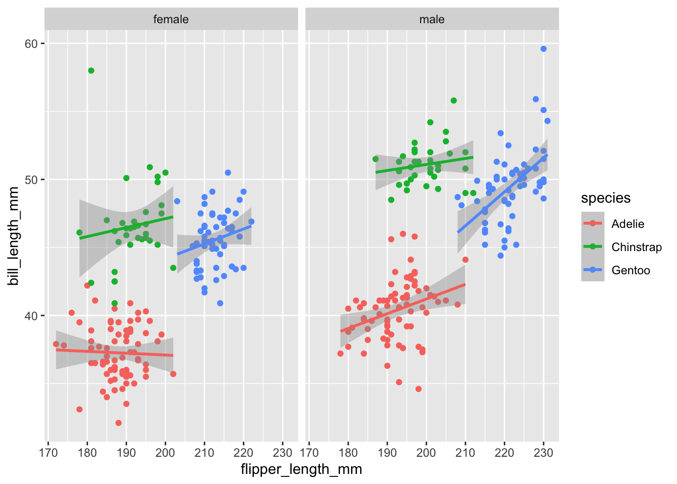

3.7.3.3 Changing the theme

The default theme for ggplot2 uses the gray background with white grid lines.

If you don’t find this suitable, you can use the black and white theme by using the theme_bw() function.

The theme_bw() function also allows you to set the typeface for the plot, in case you don’t want the default Helvetica. Here we change the typeface to Times.

For things that only make sense globally, use theme(), i.e. theme(legend.position = "none"). Two standard appearance themes are included

theme_gray(): The default theme (gray background)
theme_bw(): More stark/plain

g + 
  geom_point() + 
  geom_smooth(method = "lm") + 
  theme_bw(base_family = "Times")

Warning: Removed 2 rows containing non-finite values (`stat_smooth()`).

Warning: Removed 2 rows containing missing values (`geom_point()`).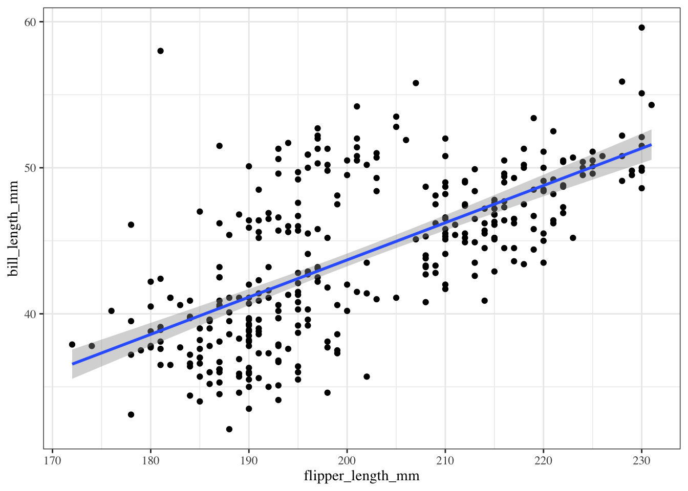

3.7.3.4 Modifying labels

There are a variety of annotations you can add to a plot, including different kinds of labels.

xlab() for x-axis labels
ylab() for y-axis labels
ggtitle() for specifying plot titles

labs() function is generic and can be used to modify multiple types of labels at once

:::

Here is an example of modifying the title and the x and y labels to make the plot a bit more informative.

g + 
  geom_point() + 
  geom_smooth(method = "lm") + 
  labs(title = "Palmer penguins", 
       x = "flipper length", 
       y = "bill length")

Warning: Removed 2 rows containing non-finite values (`stat_smooth()`).

Warning: Removed 2 rows containing missing values (`geom_point()`).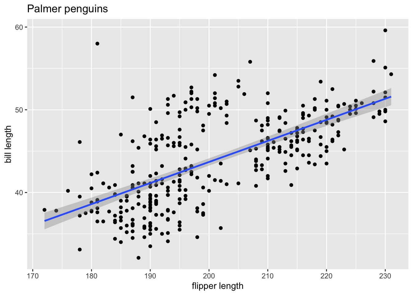

3.8 Session Info

sessionInfo()

R version 4.2.2 (2022-10-31)
Platform: aarch64-apple-darwin21.6.0 (64-bit)
Running under: macOS Ventura 13.0.1

Matrix products: default
BLAS:   /opt/homebrew/Cellar/openblas/0.3.21/lib/libopenblasp-r0.3.21.dylib
LAPACK: /opt/homebrew/Cellar/r/4.2.2/lib/R/lib/libRlapack.dylib

locale:
[1] en_US.UTF-8/en_US.UTF-8/en_US.UTF-8/C/en_US.UTF-8/en_US.UTF-8

attached base packages:
[1] stats     graphics  grDevices utils     datasets  methods   base     

other attached packages:
 [1] palmerpenguins_0.1.1 here_1.0.1           forcats_0.5.2       
 [4] stringr_1.4.1        dplyr_1.0.10         purrr_0.3.5         
 [7] readr_2.1.3          tidyr_1.2.1          tibble_3.1.8        
[10] ggplot2_3.4.0        tidyverse_1.3.2     

loaded via a namespace (and not attached):
 [1] lattice_0.20-45     lubridate_1.9.0     assertthat_0.2.1   
 [4] rprojroot_2.0.3     digest_0.6.30       utf8_1.2.2         
 [7] R6_2.5.1            cellranger_1.1.0    backports_1.4.1    
[10] reprex_2.0.2        evaluate_0.18       httr_1.4.4         
[13] highr_0.9           pillar_1.8.1        rlang_1.0.6        
[16] googlesheets4_1.0.1 readxl_1.4.1        rstudioapi_0.14    
[19] Matrix_1.5-3        rmarkdown_2.18      splines_4.2.2      
[22] labeling_0.4.2      googledrive_2.0.0   htmlwidgets_1.5.4  
[25] bit_4.0.5           munsell_0.5.0       broom_1.0.1        
[28] compiler_4.2.2      modelr_0.1.10       xfun_0.35          
[31] pkgconfig_2.0.3     mgcv_1.8-41         htmltools_0.5.3    
[34] tidyselect_1.2.0    fansi_1.0.3         crayon_1.5.2       
[37] tzdb_0.3.0          dbplyr_2.2.1        withr_2.5.0        
[40] grid_4.2.2          nlme_3.1-160        jsonlite_1.8.3     
[43] gtable_0.3.1        lifecycle_1.0.3     DBI_1.1.3          
[46] magrittr_2.0.3      scales_1.2.1        cli_3.4.1          
[49] stringi_1.7.8       vroom_1.6.0         farver_2.1.1       
[52] fs_1.5.2            xml2_1.3.3          ellipsis_0.3.2     
[55] generics_0.1.3      vctrs_0.5.1         tools_4.2.2        
[58] bit64_4.0.5         glue_1.6.2          hms_1.1.2          
[61] parallel_4.2.2      fastmap_1.1.0       yaml_2.3.6         
[64] timechange_0.1.1    colorspace_2.0-3    gargle_1.2.1       
[67] rvest_1.0.3         knitr_1.41          haven_2.5.1

3.1 Learning objectives

3.2 Reading and writing data

3.2.1 Relative paths

3.2.2 The here package

3.2.3 The readr package

3.3 Data frames and tibbles

3.3.1 Tibbles

3.3.2 How tibbles differ from data.frame

3.3.3 as_tibble()

3.4 The dplyr package

3.4.1 dplyr grammar

3.4.2 dplyr installation

3.5 dplyr functions

3.5.1 select()

3.5.2 filter()

3.5.3 arrange()

3.5.4 rename()

3.5.5 mutate()

3.5.6 group_by()

3.5.7 %>%

3.5.8 slice_*()

3.6 The ggplot2 Plotting System

3.6.1 Basic components of a ggplot2 plot

3.7 Building up in layers

3.7.1 palmerpenguins dataset

3.7.2 First plot with point layer

3.7.3 Adding more layers

3.7.3.1 smooth

3.7.3.2 facets

3.7.3.3 Changing the theme

3.7.3.4 Modifying labels

3.8 Session Info

3.2.2 The `here` package

3.2.3 The `readr` package

3.3.2 How tibbles differ from `data.frame`

3.3.3 `as_tibble()`

3.4 The `dplyr` package

3.4.1 `dplyr` grammar

3.4.2 `dplyr` installation

3.5 `dplyr` functions

3.5.1 `select()`

3.5.2 `filter()`

3.5.3 `arrange()`

3.5.4 `rename()`

3.5.5 `mutate()`

3.5.6 `group_by()`

3.5.7 `%>%`

3.5.8 `slice_*()`

3.7.1 `palmerpenguins` dataset